P.15 Carry and Tail Risk

P.15 Carry and Tail Risk#

Project Statement#

In the spring of 2007, Goldman Sachs’s Global Alpha fund — a $12 billion quantitative strategy built heavily on carry trades — began hemorrhaging money. By August, the fund had lost 22% in a single month as carry positions across currencies, credit, and rates unwound simultaneously. The pattern repeated on a global scale in 2008: strategies that had earned steady income for years collapsed in weeks. The carry trade, sometimes called “picking up nickels in front of a steamroller,” is one of the oldest risk premia in finance — and one of the most dangerous to lever.

Carry is the return earned from holding an asset regardless of price changes: the yield curve slope for bonds, the credit spread for corporate debt, the earnings yield for equities. Your task is to build carry strategies across five asset classes, discover which are genuinely harvesting a carry premium versus disguising exposure to known risk factors, combine and lever the surviving strategies using the Ch 8 leverage framework, and evaluate the result honestly with the Ch 9 toolkit.

Context#

What Is Carry?#

Carry is the return an investor earns from holding a position, assuming no change in the asset’s price. For a bond, carry is the coupon income net of funding cost — approximately the yield curve slope for a duration trade. For a credit instrument, carry is the spread over a risk-free or higher-quality benchmark. For equities, carry can be interpreted as the earnings yield or dividend yield in excess of the risk-free rate, or more broadly as the equity risk premium itself.

The common structure across carry strategies is a payoff that is steady and positive in normal markets — the “income” earned from bearing a risk — punctuated by sharp losses during crises. Carry strategies are implicitly short volatility: they collect a premium in calm environments and pay out when volatility spikes. This asymmetry means they can appear attractive on standard metrics (positive Sharpe ratios, smooth cumulative returns) until the tail materializes.

Carry Across Asset Classes#

This project constructs carry strategies across five asset classes:

Strategy	Long	Short / Funding	Carry Source
Term Carry	IEF (7–10Y Treasury)	Risk-free rate	Yield curve slope
Credit Carry	HYG (High Yield)	LQD (Inv Grade)	Credit spread
Equity Carry	SPY (S&P 500)	Risk-free rate	Equity risk premium
Dividend Carry	VYM (High Dividend)	VUG (Growth)	Dividend yield premium
FX Carry	CEW (EM Currency)	Risk-free rate	Interest rate differentials

Each strategy earns the “carry” — the spread between the long and short sides — in exchange for bearing a specific type of risk. Whether each strategy represents a genuine carry premium or is primarily repackaging a well-known factor exposure (equity beta, value, etc.) is a central analytical question.

Leverage and Carry: The Ch 8 Connection#

Practitioners routinely lever carry portfolios to boost returns. The Ch 8 result is that the Sharpe ratio is invariant to leverage — scaling a portfolio’s exposure does not change its risk-adjusted return. But the Sharpe ratio is a standardized moment (mean divided by standard deviation), and other standardized moments like skewness and kurtosis share this invariance property. Every non-standardized risk metric — maximum drawdown, VaR, CVaR — degrades with leverage.

This distinction matters. A carry portfolio may look attractive at 1× leverage: modest drawdowns, slightly negative skewness, a solid Sharpe. At 3× leverage, the Sharpe is unchanged, but the maximum drawdown may triple. LTCM’s convergence trades were structurally carry trades — earning small spreads on positions funded at extreme leverage. The question is not whether leverage changes the Sharpe ratio (it doesn’t) but where on the leverage frontier the risk becomes unacceptable — and whether the answer depends on which risk metric you use.

Nonlinear Payoffs and the Ch 9 Toolkit#

Because carry strategies collect steady income and pay out during crises, their payoff profile resembles selling insurance — or, equivalently, selling put options. The Treynor-Mazuy quadratic regression from Ch 9 tests for this structure: a negative quadratic coefficient ($\gamma < 0$) indicates concave market exposure, meaning the strategy participates in downturns more than in upturns. The Asness lagged-market diagnostic tests whether delayed pricing in less liquid markets (bonds, credit) inflates apparent alpha. Together, these tools reveal whether a carry strategy’s attractive headline metrics survive scrutiny.

Resources#

Course Materials#

Discussion 3.1: Risk — Volatility, drawdown, VaR, CVaR, return distributions
Discussion 6.1: Factor Pricing — Multi-factor decomposition, interpreting factor loadings
Discussion 8.1: Leverage — Leverage frontier, Sharpe invariance, nonlinear payoffs, LTCM
Discussion 9.1: Managed Funds — Alpha estimation, Sharpe ratio standard error, Asness lagged-market diagnostic, Treynor-Mazuy quadratic

External Reading#

Koijen, Moskowitz, Pedersen, and Vrugt (2018), “Carry”, Journal of Financial Economics — Comprehensive treatment of carry as a cross-asset risk premium
Lowenstein (2000), When Genius Failed — The LTCM story: convergence/carry trades at extreme leverage
Ilmanen (2011), Expected Returns, Ch 15 — Practitioner framework for understanding carry across asset classes

Data#

File	Description	Frequency	Date Range
`data/carry_etf_data.xlsx` (sheet: `total returns`)	Monthly total returns for SPY, IEF, TLT, SHY, HYG, LQD, VYM, VUG, CEW, DBV	Monthly	2006–2025 (varies by ETF; HYG from 2007, CEW from 2009)
`data/spy_forecasting_data.xlsx`	Carry signals: T10YR (10-year Treasury yield), CREDIT (high-yield spread), EP (earnings yield), VIX; risk-free rate (T3M as monthly decimal)	Monthly	1993–2025
`data/factor_pricing_data_monthly.xlsx`	Fama-French 5 factors + Momentum (MKT, SMB, HML, RMW, CMA, UMD) + risk-free rate	Monthly	1980–2025

Bloomberg data has been pre-pulled for convenience. Not all ETFs cover the same date range — your analysis should handle sample differences appropriately.

Data Preview#

import pandas as pd
import numpy as np
import matplotlib.pyplot as plt
import statsmodels.api as sm
import warnings
warnings.filterwarnings('ignore')

DATAPATH = '../../../data/'

# --- Load ETF total returns ---
etf_rets = pd.read_excel(f'{DATAPATH}carry_etf_data.xlsx',
                         sheet_name='total returns', index_col=0, parse_dates=True)

# --- Load carry signals and risk-free rate ---
signals = pd.read_excel(f'{DATAPATH}spy_forecasting_data.xlsx',
                        sheet_name='signals', index_col=0, parse_dates=True)
rf = pd.read_excel(f'{DATAPATH}spy_forecasting_data.xlsx',
                   sheet_name='risk-free rate', index_col=0, parse_dates=True)['T3M']

# --- Load pricing factors ---
factors = pd.read_excel(f'{DATAPATH}factor_pricing_data_monthly.xlsx',
                        sheet_name='factors (excess returns)', index_col=0, parse_dates=True)

# Sample overview
print('ETF return series:')
for col in etf_rets.columns:
    s = etf_rets[col].dropna()
    print(f'  {col:4s}: {s.index[0].strftime("%Y-%m")} to {s.index[-1].strftime("%Y-%m")} ({len(s)} months)')
print(f'\nCarry signals: {list(signals.columns)}')
print(f'Signal range: {signals.index[0].strftime("%Y-%m")} to {signals.index[-1].strftime("%Y-%m")}')

ETF return series:
  SPY : 2006-02 to 2025-06 (233 months)
  IEF : 2006-02 to 2025-06 (233 months)
  TLT : 2006-02 to 2025-06 (233 months)
  SHY : 2006-02 to 2025-06 (233 months)
  HYG : 2007-05 to 2025-06 (218 months)
  LQD : 2006-02 to 2025-06 (233 months)
  DBV : 2006-10 to 2023-03 (198 months)
  VYM : 2006-12 to 2025-06 (223 months)
  CEW : 2009-06 to 2025-12 (199 months)
  VUG : 2004-02 to 2025-12 (263 months)

Carry signals: ['DP', 'EP', 'CAPE', 'BP', 'T10YR', 'CREDIT', 'VIX']
Signal range: 1993-02 to 2025-10

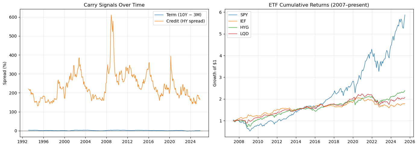
fig, axes = plt.subplots(1, 2, figsize=(14, 5))

# Panel 1: Carry signals
ax = axes[0]
common_idx = signals.index.intersection(rf.index)
term_signal = signals.loc[common_idx, 'T10YR'] - rf.loc[common_idx] * 12 * 100
credit_signal = signals.loc[common_idx, 'CREDIT']
ax.plot(term_signal.index, term_signal, label='Term (10Y − 3M)', linewidth=1)
ax.plot(credit_signal.index, credit_signal, label='Credit (HY spread)', linewidth=1)
ax.axhline(0, color='black', linewidth=0.5)
ax.set_ylabel('Spread (%)')
ax.set_title('Carry Signals Over Time')
ax.legend()
ax.grid(True, alpha=0.3)

# Panel 2: Cumulative returns of key ETFs
ax = axes[1]
start = '2007-05'
for name in ['SPY', 'IEF', 'HYG', 'LQD']:
    r = etf_rets[name].loc[start:].dropna()
    cum = (1 + r).cumprod()
    ax.plot(cum.index, cum, label=name, linewidth=1)
ax.set_ylabel('Growth of $1')
ax.set_title('ETF Cumulative Returns (2007–present)')
ax.legend()
ax.grid(True, alpha=0.3)

plt.tight_layout()
plt.show()

../_images/3d77dc3b9482ae4bb0c237688c027c854a70317e9cefd09f424a8d87cb4b2e7a.png

Questions#

Q1: Measuring Carry Signals#

Compute three carry signals from the provided data:

(a) Term carry signal: the yield spread between 10-year Treasuries and 3-month T-bills (T10YR minus the annualized risk-free rate, T3M × 12 × 100 to convert to percentage points). Credit carry signal: the high-yield credit spread (CREDIT in the signals data). Equity carry signal: the earnings yield in excess of the annualized risk-free rate (EP minus the annualized risk-free rate).

(b) Plot all three signals over time on separate panels. Annotate major crisis episodes: the 2008 GFC, the 2011 European debt crisis, the 2020 COVID crash, and the 2022 rate hiking cycle.

(c) Discuss the relationship between carry signal levels and crisis episodes. What does the pattern tell you about what carry compensates for?

Q2: Building the Carry Strategy Universe#

(a) Construct the five carry strategies described in the Context section using the ETF total returns and risk-free rate data. Compute monthly return series for each.

(b) Report annualized return, volatility, Sharpe ratio, maximum drawdown, skewness, and kurtosis in a single summary table. Use the common sample period across all five strategies. Also report the pairwise correlation matrix.

(c) Discuss what the performance metrics and correlations reveal about the nature of carry returns across these asset classes.

Q3: Crisis Correlations and Diversification#

(a) Define a set of “crisis months” using a criterion you consider appropriate and justify your choice. Compute the pairwise correlation matrix across all five carry strategies separately for crisis and non-crisis months.

(b) Construct an equal-weight portfolio of all five carry strategies. Report its annualized return, volatility, Sharpe ratio, and maximum drawdown separately for crisis and non-crisis subsamples.

(c) How does diversification across carry asset classes hold up during stress?

Q4: Factor Decomposition and Strategy Curation#

(a) Regress each of the five carry strategies on the Fama-French five factors plus momentum (MKT, SMB, HML, RMW, CMA, UMD). Report the factor loadings with t-statistics, the $R^2$, and the annualized intercept (alpha).

(b) Based on the full set of evidence from Q2–Q4 — performance metrics, crisis correlations, and factor exposures — select a subset of strategies that represent genuine, non-redundant carry premia. Drop any strategy that is primarily repackaging a known factor exposure or is too correlated with another to provide meaningful diversification. Justify your choices explicitly.

(c) Construct a curated equal-weight carry portfolio from the surviving strategies. This portfolio is the subject of Q5–Q7.

Q5: The Leverage Frontier#

Scale your curated carry portfolio from Q4 to leverage levels from 0.5× to 3.0× (in increments of 0.5×). At each level, compute: annualized return, volatility, Sharpe ratio, maximum drawdown, skewness, and kurtosis.

(a) Plot the leverage frontier: Sharpe ratio vs. leverage on one panel, maximum drawdown on another. Which risk metrics are invariant to leverage, and which are not?

(b) Construct a vol-targeted version: each month, set leverage so that the trailing 12-month realized volatility equals 10% annualized. Compare its performance metrics to the fixed-leverage versions. Examine the leverage time series.

(c) Compute the worst single-month return at 1× leverage. Scale that loss to higher leverage multiples. At what point does a single bad month become existential?

Q6: Evaluating the Carry Portfolio#

Apply the Ch 9 evaluation toolkit to your curated carry portfolio at 1× leverage.

(a) Estimate alpha against MKT alone, then against the full FF5 + UMD model. Report coefficients with t-statistics.

(b) Compute the Sharpe ratio standard error:

\[SE(\widehat{SR}) = \sqrt{\frac{1 + \widehat{SR}^2 / 2}{T}}\]

Report the 95% confidence interval. How many years of data would you need before the carry premium is statistically distinguishable from zero?

(c) Run two diagnostic regressions: (i) the Asness lagged-market test — regress excess returns on the contemporaneous and one-month lagged market return; (ii) the Treynor-Mazuy quadratic test — regress excess returns on MKT and MKT$^2$. Report and interpret the results.

Q7: Synthesis#

A pension fund CIO asks: “We want to add a diversified carry portfolio at 1.5× leverage to target our return objective. What should we know?”

Write a concise assessment (2–3 paragraphs) grounded in your specific findings from Q1–Q6 — not general principles, but the numbers you computed.

Deliverables#

Review the Project Guidelines for submission standards, conciseness expectations, and AI usage policy.

Submit a single Jupyter notebook containing code, output, and written analysis for Q1–Q7.

Include a summary table comparing all carry strategies and the curated portfolio on: annualized return, volatility, Sharpe ratio (with SE), maximum drawdown, skewness, and alpha.

Conciseness is a graded criterion — see Project Guidelines.