MV Optimization Details#
Portfolio Fundamentals#
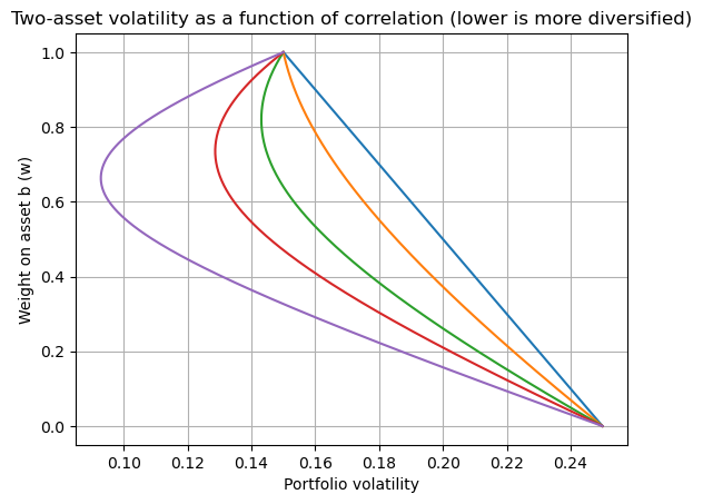
The risk of a portfolio is a nonlinear function of asset risks: covariances matter. Optimal portfolios either (i) maximize expected return for a given risk or (ii) minimize risk for a given return.
Portfolio mean and variance; diversification#
For two assets with weights \(w\) and \(1-w\): $\( \mu_p = w \, \mu_b + (1-w)\, \mu_s \)\( \)\( \sigma_p^2 = w^2 \sigma_b^2 + (1-w)^2 \sigma_s^2 + 2w(1-w)\rho \sigma_b \sigma_s \)$
Volatility is linear in weights only if \(\rho = 1\).
Diversification occurs whenever \(\rho < 1\) (it does not require \(\rho \le 0\)).
import numpy as np
import matplotlib.pyplot as plt

mu_b, mu_s = 0.08, 0.12
sig_b, sig_s = 0.15, 0.25

ws = np.linspace(0, 1, 251)
def port_stats(w, rho):
    mu = w*mu_b + (1-w)*mu_s
    var = (w**2)*(sig_b**2) + ((1-w)**2)*(sig_s**2) + 2*w*(1-w)*rho*sig_b*sig_s
    return mu, np.sqrt(var)

fig, ax = plt.subplots()
for rho in [1.0, 0.7, 0.3, 0.0, -0.5]:
    sigmas = [port_stats(w, rho)[1] for w in ws]
    ax.plot(sigmas, ws)  # plot risk vs weight to show curvature changes
ax.set_xlabel("Portfolio volatility")
ax.set_ylabel("Weight on asset b (w)")
ax.set_title("Two-asset volatility as a function of correlation (lower is more diversified)")
ax.grid(True)
plt.show()
Perfect hedge (\(\rho=-1\))#
With two assets and \(\rho = -1\), set weights so that \(\sigma_p=0\): $\( \frac{w_s}{w_b} = \frac{\sigma_b}{\sigma_s} \, . \)$
Diversification across n assets (general results)#
Let there be n risky assets with volatilities \(\sigma_i\) and covariances \(\sigma_{i,j}\). For portfolio weights \(w_i\) with \(\sum_i w_i = 1\), the variance is
Equally weighted case#
For \(w_i = \frac{1}{n}\),
Define the across-asset averages
Then
As \(n\to\infty\) with a diversified portfolio (no single name has material weight), the idiosyncratic term vanishes:
Identical vol and correlation#
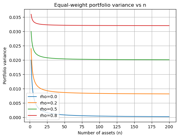
If \(\sigma_i=\sigma\) for all i and \(\rho_{i,j}=\rho\) for \(i\neq j\):
Systematic risk: \(\rho\sigma^2\)
Idiosyncratic risk: \(\frac{1}{n}\sigma^2\) (diversifiable)
Special cases:
• \(\rho=1\): no diversification, \(\sigma_p^2=\sigma^2\).
• \(\rho=0\): fully diversifiable, \(\sigma_p^2=\frac{1}{n}\sigma^2 \to 0\).
• With two assets and \(\rho=-1\), one can choose weights to make \(\sigma_p=0\).
import numpy as np
import matplotlib.pyplot as plt

np.random.seed(0)
sig2 = 0.2**2
rhos = [0.0, 0.2, 0.5, 0.8]
ns = np.arange(2, 201)

def portfolio_var_equal(n, rho, sig2=sig2):
    # identical variances and pairwise correlation rho
    return (1/n)*sig2 + ((n-1)/n)*rho*sig2

fig, ax = plt.subplots()
for rho in rhos:
    vars_ = [portfolio_var_equal(n, rho) for n in ns]
    ax.plot(ns, vars_, label=f"rho={rho}")
ax.set_xlabel("Number of assets (n)")
ax.set_ylabel("Portfolio variance")
ax.set_title("Equal-weight portfolio variance vs n")
ax.grid(True)
ax.legend()
plt.show()
Mean–Variance (MV) optimization (no risk-free asset)#
Let \(r \in \mathbb{R}^n\) denote asset returns with mean \(\mu = \mathbb{E}[r]\) and covariance \(\Sigma \succ 0\). A portfolio is \(\omega\in\mathbb{R}^n\) with \(\omega^\top \mathbf{1} = 1\).
We solve, for a target mean \(\mu_p\):
Lagrangian \(\mathcal{L} = \tfrac12 \omega^\top \Sigma \omega - \gamma_1(\omega^\top \mu - \mu_p) - \gamma_2(\omega^\top \mathbf{1}-1)\).
FOC: \(\Sigma \omega - \gamma_1 \mu - \gamma_2 \mathbf{1} = 0 \Rightarrow \omega^* = \gamma_1 \Sigma^{-1}\mu + \gamma_2 \Sigma^{-1}\mathbf{1}\).
Define the two special MV portfolios
Then every MV portfolio can be written as
for a suitable \(\delta \in \mathbb{R}\).
Here, \(\omega_v\) is the Global Minimum Variance (GMV) portfolio; \(\omega_t\) is the portfolio on the risky MV frontier whose tangent passes through the origin.
MV with a risk-free asset (excess returns, tangency, CML)#
Let \(r_f\) be the risk-free rate and define excess means \(\tilde{\mu} \equiv \mu - \mathbf{1} r_f\).
We now choose weights only on risky assets \(w\) (the remainder \(1 - \mathbf{1}^\top w\) sits in the risk-free asset).
For a target excess mean \(\tilde{\mu}_p\), solve $\( \min_{w} \ w^\top \Sigma w \quad \text{s.t.} \quad w^\top \tilde{\mu} = \tilde{\mu}_p. \)\( Solution: \)\( w^* = \tilde{\delta}\, w_t, \quad w_t \equiv \frac{\Sigma^{-1}\tilde{\mu}}{\mathbf{1}^\top \Sigma^{-1}\tilde{\mu}}, \quad \tilde{\delta} = \frac{\mathbf{1}^\top \Sigma^{-1}\tilde{\mu}}{\tilde{\mu}^\top \Sigma^{-1}\tilde{\mu}}\;\tilde{\mu}_p. \)$
Variance along the efficient line: $\( \sigma_p^2 = \frac{\tilde{\mu}_p^2}{\tilde{\mu}^\top \Sigma^{-1}\tilde{\mu}}. \)$
\(w_t\) is the tangency portfolio (100% risky, max Sharpe on the risky frontier).
The Capital Market Line (CML) is the efficient straight line through \((0, r_f)\) with slope \(\max SR = \sqrt{\tilde{\mu}^\top \Sigma^{-1}\tilde{\mu}}\).
Any efficient portfolio is a mix of \(w_t\) and the risk-free asset.
Two-fund separation#
Without a risk-free asset: any MV portfolio is a linear combination of two MV portfolios (e.g., \(\omega_t\) and \(\omega_v\)).
With a risk-free asset: any efficient portfolio is a linear combination of the tangency portfolio \(w_t\) and the risk-free asset.
Complete Implementation#
Below are complete, dependency-light helpers to compute GMV and tangency portfolios from \(\mu\) and \(\Sigma\), and to draw the risky MV frontier and the CML.
import numpy as np
import matplotlib.pyplot as plt

def gmv_weights(Sigma):
    """Global Minimum Variance portfolio weights."""
    inv = np.linalg.inv(Sigma)
    ones = np.ones(Sigma.shape[0])
    w = inv @ ones
    w = w / (ones @ inv @ ones)
    return w

def risky_tangency_weights(mu, Sigma, rf=0.0):
    """Tangency portfolio weights (risky assets only)."""
    tilde_mu = mu - rf
    inv = np.linalg.inv(Sigma)
    ones = np.ones(Sigma.shape[0])
    w = inv @ tilde_mu
    w = w / (ones @ inv @ tilde_mu)
    return w

def mv_frontier(mu, Sigma, num=100):
    """Return (sigmas, means) for the risky MV frontier (no rf)."""
    inv = np.linalg.inv(Sigma)
    ones = np.ones(Sigma.shape[0])
    phi0 = mu @ inv @ mu
    phi1 = mu @ inv @ ones
    phi2 = ones @ inv @ ones
    # Parameterize by target mean between GMV mean and a high value
    mu_gmv = (gmv_weights(Sigma) @ mu)
    mu_hi = float(max(mu_gmv*3, mu_gmv + np.sqrt(phi0)))  # heuristic span
    mus = np.linspace(mu_gmv*0.8, mu_hi, num)
    vars_ = (phi0 - 2*phi1*mus + phi2*mus**2) / (phi0*phi2 - phi1**2)
    sigs = np.sqrt(np.maximum(vars_, 0))
    return sigs, mus

def normalize_weights(w):
    """Normalize weights to sum to 1."""
    s = w.sum()
    return w / s

def mvp_weights(Sigma):
    """Minimum Variance Portfolio weights."""
    one = np.ones(Sigma.shape[0])
    w_unnorm = np.linalg.solve(Sigma, one)
    return normalize_weights(w_unnorm)

def tangency_weights(mu, Sigma):
    """Tangency portfolio weights."""
    w_unnorm = np.linalg.solve(Sigma, mu)
    return normalize_weights(w_unnorm)

def port_stats_from_w(w, mu, Sigma):
    """Portfolio statistics from weights."""
    mu_p = w @ mu
    sig_p = np.sqrt(w @ Sigma @ w)
    return mu_p, sig_p
Example: 4-asset portfolio#
# Toy example with 4 assets
mu = np.array([0.06, 0.08, 0.10, 0.12])  # expected excess returns
std = np.array([0.10, 0.15, 0.20, 0.25])
corr = np.array([
    [1.0, 0.3, 0.2, 0.1],
    [0.3, 1.0, 0.4, 0.2],
    [0.2, 0.4, 1.0, 0.5],
    [0.1, 0.2, 0.5, 1.0],
])
Sigma = np.outer(std, std) * corr

wV = mvp_weights(Sigma)
wT = tangency_weights(mu, Sigma)

print("MVP weights:", np.round(wV, 4))
print("Tangency weights:", np.round(wT, 4))

# Portfolio statistics
mu_V, sig_V = port_stats_from_w(wV, mu, Sigma)
mu_T, sig_T = port_stats_from_w(wT, mu, Sigma)

print(f"\nMVP: μ={mu_V:.4f}, σ={sig_V:.4f}")
print(f"Tangency: μ={mu_T:.4f}, σ={sig_T:.4f}")
MVP weights: [0.7125 0.1818 0.0396 0.0661]
Tangency weights: [0.5465 0.2207 0.0863 0.1466]

MVP: μ=0.0692, σ=0.0909
Tangency: μ=0.0767, σ=0.0957
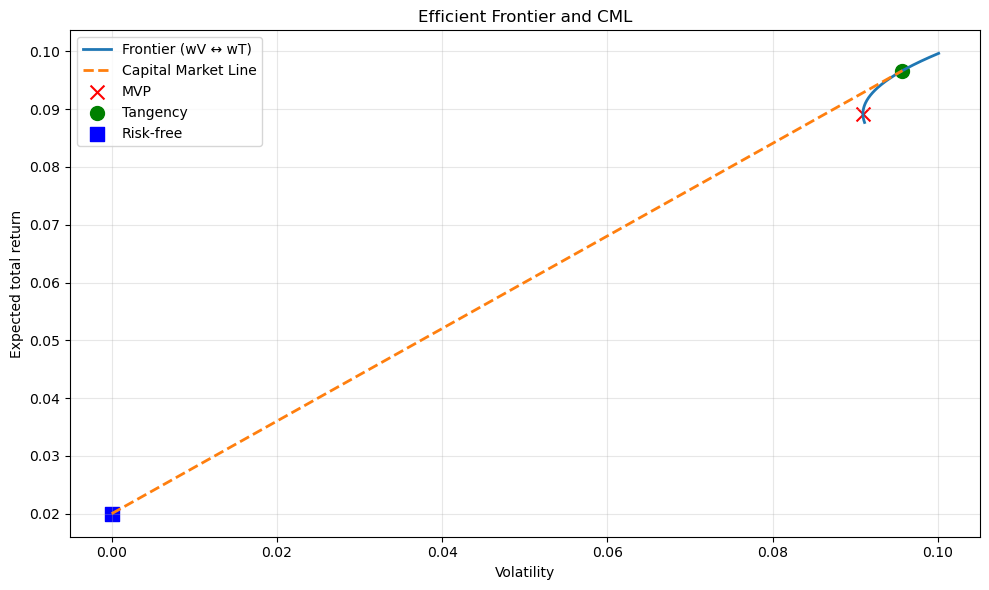
Efficient frontier visualization#
# Frontier from combining wV and wT over delta grid
deltas = np.linspace(-0.2, 1.4, 161)
mus, sigs = [], []
for d in deltas:
    w = d*wT + (1-d)*wV
    m, s = port_stats_from_w(w, mu, Sigma)
    mus.append(m)
    sigs.append(s)

# Risk-free rate
rf = 0.02
# Translate to total return space for the plot: add rf back to excess return means
total_mus = np.array(mus) + rf
total_rf = rf

# CML: line through (0, rf) and the tangency point in total-return space
mu_T_excess, sig_T = port_stats_from_w(wT, mu, Sigma)
mu_T_total = mu_T_excess + rf

fig, ax = plt.subplots(figsize=(10, 6))
ax.plot(sigs, total_mus, label="Frontier (wV ↔ wT)", linewidth=2)
ax.plot([0, sig_T], [total_rf, mu_T_total], label="Capital Market Line", linewidth=2, linestyle='--')
ax.scatter([sig_V], [mu_V + rf], marker="x", s=100, label="MVP", color='red')
ax.scatter([sig_T], [mu_T_total], marker="o", s=100, label="Tangency", color='green')
ax.scatter([0], [rf], marker="s", s=100, label="Risk-free", color='blue')
ax.set_xlabel("Volatility")
ax.set_ylabel("Expected total return")
ax.set_title("Efficient Frontier and CML")
ax.grid(True, alpha=0.3)
ax.legend()
plt.tight_layout()
plt.show()
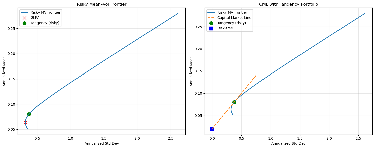
Advanced example: 6-asset portfolio with CML#
# --- Advanced example (replace with your estimates) ---
np.random.seed(0)
n = 6
A = np.random.randn(n, n)
Sigma = A @ A.T / n + 0.05*np.eye(n)   # PD covariance
mu = np.linspace(0.03, 0.12, n)        # ascending means
rf = 0.02

w_gmv = gmv_weights(Sigma)
w_tan = risky_tangency_weights(mu, Sigma, rf=rf)

sig_risky, mu_risky = mv_frontier(mu, Sigma, num=200)

# Risk-free mix line (CML): line through (sigma=0, mean=rf) tangent at risky tangency point
tan_sigma = float(np.sqrt(w_tan @ Sigma @ w_tan))
tan_mean = float(w_tan @ mu)
cml_sigmas = np.linspace(0, tan_sigma*2, 100)
# Slope is Sharpe of tangency: (tan_mean - rf) / tan_sigma
cml_means = rf + (tan_mean - rf) / tan_sigma * cml_sigmas

# --- Plot 1: Risky MV frontier ---
fig, (ax1, ax2) = plt.subplots(1, 2, figsize=(15, 6))

ax1.plot(sig_risky, mu_risky, label="Risky MV frontier", linewidth=2)
ax1.scatter([np.sqrt(w_gmv @ Sigma @ w_gmv)], [w_gmv @ mu], marker="x", s=100, label="GMV", color='red')
ax1.scatter([tan_sigma], [tan_mean], marker="o", s=100, label="Tangency (risky)", color='green')
ax1.set_xlabel("Annualized Std Dev")
ax1.set_ylabel("Annualized Mean")
ax1.legend()
ax1.set_title("Risky Mean–Vol Frontier")
ax1.grid(True, alpha=0.3)

# --- Plot 2: Capital Market Line (with rf) ---
ax2.plot(sig_risky, mu_risky, label="Risky MV frontier", linewidth=2)
ax2.plot(cml_sigmas, cml_means, label="Capital Market Line", linewidth=2, linestyle='--')
ax2.scatter([tan_sigma], [tan_mean], marker="o", s=100, label="Tangency (risky)", color='green')
ax2.scatter([0], [rf], marker="s", s=100, label="Risk-free", color='blue')
ax2.set_xlabel("Annualized Std Dev")
ax2.set_ylabel("Annualized Mean")
ax2.legend()
ax2.set_title("CML with Tangency Portfolio")
ax2.grid(True, alpha=0.3)

plt.tight_layout()
plt.show()

print("GMV weights:", np.round(w_gmv, 4))
print("Tangency (risky) weights:", np.round(w_tan, 4))
print("Tangency Sharpe:", np.round((tan_mean - rf)/tan_sigma, 4))
GMV weights: [ 0.0449  0.4636  0.382   0.0771 -0.2622  0.2946]
Tangency (risky) weights: [ 0.0788  0.2255  0.294   0.0723 -0.1107  0.4401]
Tangency Sharpe: 0.1602
References#
Back, Asset Pricing and Portfolio Choice Theory, Ch. 5.
Bodie, Kane, and Marcus, Investments, Ch. 7.