Risk and Return Metrics

import pandas as pd
import numpy as np
import datetime
import warnings

import matplotlib.pyplot as plt
%matplotlib inline
plt.rcParams['figure.figsize'] = (8,4)
plt.rcParams['font.size'] = 13
plt.rcParams['legend.fontsize'] = 13

from matplotlib.ticker import (MultipleLocator,
                               FormatStrFormatter,
                               AutoMinorLocator)

from sklearn.linear_model import LinearRegression

from cmds.portfolio import *
from cmds.risk import *
from cmds.plot_tools import plot_triangular_matrix

LOADFILE = '../data/risk_etf_data.xlsx'
info = pd.read_excel(LOADFILE,sheet_name='descriptions').set_index('ticker')
rets = pd.read_excel(LOADFILE,sheet_name='total returns').set_index('Date')
prices = pd.read_excel(LOADFILE,sheet_name='prices').set_index('Date')

FREQ = 252

Risk

Volatility or More?

What is meant by risk?

May be associated with

• loss

• volatility

• correlation

• worst outcomes

• sensitivity

Various risk measures try to give information on all these.

Return, Price, PnL, Other?

Our discussion of risk will be general to any asset class.

• Examples are across various assets.

The object of analysis will depend on the asset class:

• bonds and options: price

• equities, futures, and currency: return

At times, it will make sense to examine profit and loss (PnL).

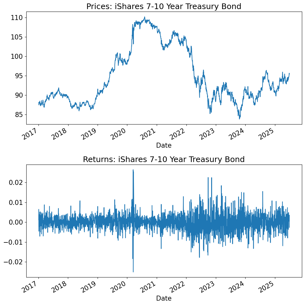
TICK = 'IEF'
fig, ax = plt.subplots(2,1,figsize=(10,10))
desc = info.loc[TICK,'shortName']
prices[TICK].plot(ax=ax[0],title=f'Prices: {desc}')
rets[TICK].plot(ax=ax[1],title=f'Returns: {desc}')
plt.tight_layout()
plt.show()

Tools

The tools used are different than fixed income and options pricing. Relatively

• more statistics

• less math

For bonds and options, we saw risk via

• mathematical sensitivity of prices

For equities and other assets, we will be using

• statistical sensitivity of returns (or scaled prices)

Model Approach

The modeling approach will rely on formulating the data such that it is

• stationary

  • Nearly always

  • This is often the motive for switching between prices, profits, returns, etc.

• iid (indepently and identically distributed)

  • Much of the complication is achieving this.

• normally distributed?

  • Rarely required.

  • A useful comparison.

  • At times a simplfiying approximation

Note: Difference to Pricing

Risk uses different tools than pricing.

• No alternative probability measures.

• Volatility will mean actual variation, not options pricing quotes.

• Mostly use discrete-time models, not continuous-time stochastic calculus.

Starting Point

Question:

• Is a 10-year Treasury Note risky?

To start, we consider risk over a single given period.

• This is not just pedagogical

• Risk managers will mostly focus on risk over the next period.

• Delta, duration are good examples of this

For some problems, we will need to consider

• multiple-period risk

• cumulative returns

Moments

Data

As an example for analyzing risk, we consider

• ETF data on various asset classes

• daily frequency

• 2017 through present

The ETF data ensures

• we are looking at traded security returns, not indexes

• thus, no issue of rolling futures, carry on FX, etc.

• Though there may be differences due to fund expenses and fund tracking error (oil?)

info

	quoteType	shortName	volume	totalAssets	longBusinessSummary
ticker
SPY	ETF	SPDR S&P 500	91993247	6.035170e+11	The trust seeks to achieve its investment obje...
VEA	ETF	Vanguard FTSE Developed Markets	14117842	2.247459e+11	The fund employs an indexing investment approa...
UPRO	ETF	ProShares UltraPro S&P 500	3575899	3.852897e+09	The fund invests in financial instruments that...
GLD	ETF	SPDR Gold Trust	8046469	9.798884e+10	The Trust holds gold bars and from time to tim...
USO	ETF	United States Oil Fund	5910069	9.070093e+08	USO invests primarily in futures contracts for...
FXE	ETF	Invesco CurrencyShares Euro Cur	195591	5.239969e+08	NaN
BTC-USD	CRYPTOCURRENCY	Bitcoin USD	41706745856	NaN	NaN
HYG	ETF	iShares iBoxx $ High Yield Corp	49277832	1.594403e+10	The underlying index is a rules-based index co...
IEF	ETF	iShares 7-10 Year Treasury Bond	10542291	3.493820e+10	The underlying index measures the performance ...
TIP	ETF	iShares TIPS Bond ETF	4252748	1.390087e+10	The index tracks the performance of inflation-...
SHV	ETF	iShares Short Treasury Bond ETF	3521474	2.059998e+10	The fund will invest at least 80% of its asset...

Mean

The mean is the first moment of the (unspecified) distribution:

\[ \mu = \E[r]\]

The sample estimator for it is

\[\meanest = \frac{1}{\Ntime}\sum_{t=1}^\Ntime r_t\]

Note that this is often expressed with “bar” notation, \(\bar{r}\).

• Here the notation is \(\hat{\mu}\) for symmetry with many estimators below using “hat” notation.

Important for risk?

For measuring and analyzing risk, we will mostly consider de-meaned data.

• We want to know the possible outcomes relative to the mean.

• Interesting models of the mean are more useful for forecasting returns for directional investing.

Note

• Having an incorrect measure of the mean will cause error in our relative assessments.

• However, the main focus will be risk over short periods, for which the mean (trend) will not matter much to the calculation.

Data: Means

The mean ETF data is listed below for price an return.

Technical Note

• Does it make sense to analyze this for price and return?

• That is, do they both satisfy basic statistical properties to be well-suited to examining unconditional moments?

pd.concat([prices.mean(),rets.mean()*FREQ],axis=1,keys=['price','return']).style.format({'price':'{:.2f}','return':'{:.2%}'})

	price	return
SPY	359.07	15.29%
VEA	39.58	9.70%
UPRO	40.94	38.85%
GLD	166.55	12.88%
USO	73.74	5.02%
FXE	101.46	1.60%
BTC	29104.00	79.29%
HYG	65.85	4.65%
IEF	94.75	1.26%
TIP	100.05	2.76%
SHV	97.95	2.16%

Variance and Volatility (StdDev)

The variance is the second centered moment of the (unspecified) distribution.

\[\sigma^2 = \E\left[(r-\mu)^2\right]\]

The usual sample estimator for the variance is

\[\hat{\sigma}^2 = \frac{1}{\Ntime-1}\sum_{t=1}^\Ntime(r_t-\meanest)^2\]

Question

Note that though there are \(\Ntime\) data points in the sample, the estimator for the variance uses \(\Ntime-1\).

What is the reason?

• statistically

• conceptually

Standard Deviation

The standard deviation (in population and in sample) is the square root of the formulas above.

• We will often refer to this as the volatility.

• One could make the distinction of volatility as the time-varying (instantaneous) standard deviation of the process, but more often it is used synonomously with standard deviation.

Technical Points

Non-negativity

The standard deviation is defined in such a way that it is always non-negative.

• Thus, models of volatility (realized: GARCH, implied: SABR) have to be careful to ensure this holds.

Centering

The variance is the second squared moment. Note that inside the expectation is \(r-\mu\).

The second (uncentered) moment is \(\E\left[r^2\right]\), and it is sometimes useful to have the variance as the difference of the (uncentered) first and second moments:

\[\sigma^2 = \E\left[r^2\right] - \left(\E[r]\right)^2\]

vol = (rets.std().to_frame('vol')*np.sqrt(FREQ))
vol['variance'] = vol['vol']**2
vol.style.format('{:.2%}')

	vol	variance
SPY	18.85%	3.55%
VEA	17.51%	3.06%
UPRO	56.49%	31.92%
GLD	14.28%	2.04%
USO	38.60%	14.90%
FXE	7.37%	0.54%
BTC	69.83%	48.77%
HYG	8.68%	0.75%
IEF	6.88%	0.47%
TIP	6.02%	0.36%
SHV	0.28%	0.00%

Higher Moments

Skewness

Skewness is the third moment (centered and scaled).

\[\varsigma = \frac{1}{\sigma^3}\E\left[(r-\mu)^3\right]\]

The sample estimator is

\[\hat{\varsigma} = \frac{1}{\hat{\sigma}^3} \frac{1}{\Ntime-1}\sum_{t=1}^\Ntime(r_t-\meanest)^3\]

Note that the skewness

• can be positive or negative

• is NOT typically listed as a percentage

The skewness is negative for distributions where there is an asymmetric, “long left tail”.

Kurtosis

Kurtosis is the fourth moment (centered and scaled).

\[\kappa = \frac{1}{\sigma^4}\E\left[(r-\mu)^4\right]\]

The sample estimator is

\[\hat{\kappa} = \frac{1}{\hat{\sigma}^4} \frac{1}{\Ntime-1}\sum_{i=1}^\Ntime(r_t-\meanest)^4\]

Note that the kurtosis

• is non-negative

• is NOT typically listed as a percentage

Furthermore, kurtosis is typically expressed excess kurtosis, \(\kappa - 3\).

• This is to compare it to the normal distribution, which has kurtosis of 3.

The skewness is negative for distributions where there is an asymmetric, “long left tail”.

get_moments(rets,FREQ)

	mean	vol	skewness	kurtosis
SPY	15.3%	18.9%	-0.30	14.24
VEA	9.7%	17.5%	-0.86	16.12
UPRO	38.8%	56.5%	-0.38	14.99
GLD	12.9%	14.3%	-0.15	2.70
USO	5.0%	38.6%	-1.28	16.30
FXE	1.6%	7.4%	0.16	1.35
BTC	79.3%	69.8%	0.03	6.15
HYG	4.6%	8.7%	0.13	26.42
IEF	1.3%	6.9%	0.20	3.20
TIP	2.8%	6.0%	0.36	14.86
SHV	2.2%	0.3%	0.66	3.28

Annualizing the Moments

To annualize the moments use the frequency, of data per year, \(\tau\),

	annualize	sign	quote
mean	\(\tau\)	+ / -	%
volatility	\(\sqrt{\tau}\)	+	%
skewness	1	+ / -	number
kurtosis	1	+	number

For instance, to annualize (trading)

• daily data, \(\tau=252\).

• monthly data, \(\tau=12\).

Distribution

Quantiles

The risk measures based on “moments” make use of data in the entire distribution.

• This allows for high statistical power.

• Those moments make no assumption about the distribution.

The quantiles

• continue without any assumption on the distribution.

But they are estimating a single point on the distribution.

• This means it gets less precision from the sample.

If the variable has a distribution with a continuous and strictly increasing cdf, denoted \(F\), with an inverse cdf of \(F^{-1}\). Then the quantile \(\pi\) is $\(q_{\pi} = F^{-1}(\pi)\)$

The sample estimate is the order statistic.

• Sort the sample into ascending order.

• Define the sorted data as \(\{r_{(1)},\ldots,r_{(\Ntime)}\}\).

\[\hat{q}_{\pi} = r_{(\pi \Ntime)}\]

Median

Of course, for \(\pi=0.5\), this is the median:

\[\hat{q}_{0.5} = r_{\text{median}}\]

Technical Note

If \(\pi\Ntime\) is not an integer, typical to take a linear interpretation between the nearest two ordered points.

\[\hat{q}_{\pi} = \frac{r_{(\pi \Ntime-)} + r_{(\pi \Ntime+)}}{2}\]

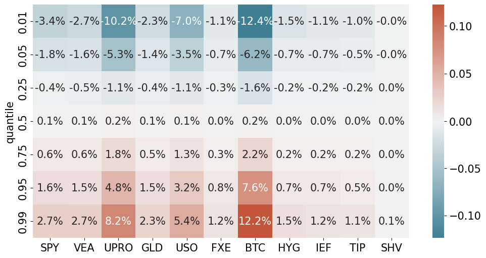
from matplotlib.colors import TwoSlopeNorm

quantiles = rets.quantile(q=[.01,.05,.25,.5,.75,.95,.99])
quantiles.index.name = 'quantile'

quantiles.reset_index(inplace=True)
quantiles['quantile'] = quantiles['quantile'].astype(str)
quantiles.set_index('quantile',inplace=True)
quantiles.style.format('{:.1%}')

# Create a diverging colormap centered at 0
colors = sns.diverging_palette(220, 20, as_cmap=True)

# Plot heatmap with twoslope normalization
sns.heatmap(quantiles, 
            annot=True, 
            fmt='.1%',
            cmap=colors,
            norm=TwoSlopeNorm(vmin=quantiles.min().min(), 
                             vcenter=0, 
                             vmax=quantiles.max().max()))
plt.show()

Normal Distribution

NONE of the measures discussed above rely on a normal distribution.

But later we will consider estimates that rely on an assumed distribution, and whether returns are normal.

So how good of an approximation is a normal distribution?

data = rets['SPY']
fig = plot_normal_histogram(data,bins=250);
plt.title('Histogram of Returns');
plt.show()

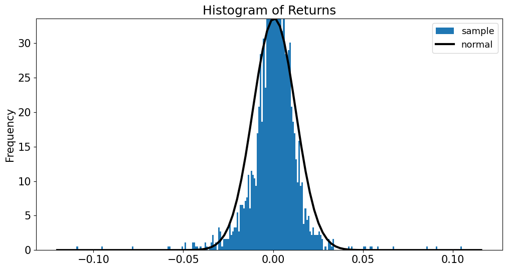
Outliers

The histogram doesn’t look too far off at first glance.

But consider the outliers.

• A normal distribution implies 5 and 10 std.dev. outliers almost never happen.

• In the sample above, there are numerous.

Outlier Table

• The outlier table below shows z-scores for the min and max return.

• The final two columns show the probability of such values happening under a normal distribution.

outlier_normal(rets).set_caption('Daily')

Daily

	z min	z max	normal prob min	normal prob max
SPY	-9.27	8.79	9.66e-21	0.00e+00
VEA	-10.17	8.03	1.31e-24	4.44e-16
UPRO	-9.86	7.81	3.01e-23	2.78e-15
GLD	-6.03	5.34	8.33e-10	4.66e-08
USO	-10.42	6.85	1.00e-25	3.78e-12
FXE	-4.44	5.34	4.45e-06	4.58e-08
BTC	-8.52	5.67	7.91e-18	7.23e-09
HYG	-10.08	11.94	3.23e-24	0.00e+00
IEF	-5.80	6.09	3.36e-09	5.82e-10
TIP	-7.59	11.72	1.61e-14	0.00e+00
SHV	-5.16	6.25	1.27e-07	2.06e-10

Astronomical

The probabilities are astronomical.

• Clearly the returns are not normally distributed–particularly for tail events.

Ironically, this means that a normal distribution as a rough approximation might be fine–except for the events we care most about in managing risk–big outliers.

Time Frequency

However, consider that the normality may depend on the frequency of the data.

• At finer granularity, (daily, intra-daily,) perhaps the aberrations are stronger.

• At a less frequent time interval, perhaps these compound and average out.

Monthly returns

The table below repeats the example for monthly returns.

retsM = prices.resample('M').last().pct_change()
outlier_normal(retsM).set_caption('Monthly')

/var/folders/zx/3v_qt0957xzg3nqtnkv007d00000gn/T/ipykernel_7584/1399536021.py:1: FutureWarning: 'M' is deprecated and will be removed in a future version, please use 'ME' instead.
  retsM = prices.resample('M').last().pct_change()

Monthly

	z min	z max	normal prob min	normal prob max
SPY	-2.96	2.48	1.52e-03	6.65e-03
VEA	-3.46	2.94	2.72e-04	1.63e-03
UPRO	-3.56	2.38	1.88e-04	8.64e-03
GLD	-2.15	2.57	1.58e-02	5.11e-03
USO	-4.92	3.06	4.26e-07	1.11e-03
FXE	-2.39	2.55	8.51e-03	5.36e-03
BTC	-1.95	2.85	2.59e-02	2.20e-03
HYG	-4.58	2.78	2.36e-06	2.73e-03
IEF	-2.47	2.27	6.74e-03	1.15e-02
TIP	-4.55	2.68	2.71e-06	3.73e-03
SHV	-1.52	1.90	6.44e-02	2.85e-02

Maximum Drawdown

The maximum drawdown (MDD) of a return series is the maximum cumulative loss suffered during the time period.

• Visually, this is the largest peak-to-trough during the sample.

• It is widely cited in performance evaluation to understand how badly the investment might perform.

Technical Note

Maximum drawdown is widely cited in backtests.

• This can be quite useful in understanding the scale / nature of the strategy, especially how it performs in certain scenarios.

• It is less useful than the “moment” statistics above in forecasting the future.

• It is a path-dependent statistic, and it has much less statistical precision.

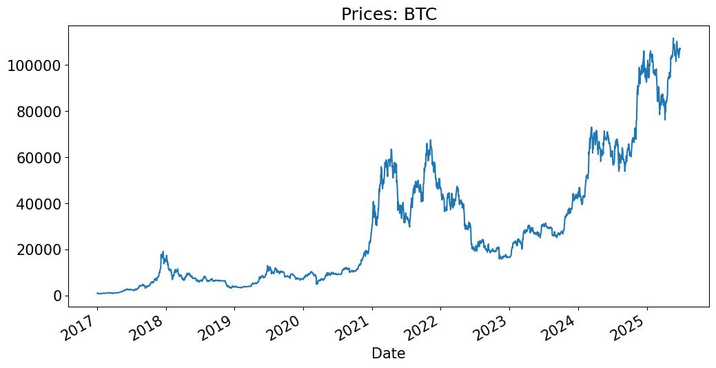
Example

Consider the price chart below.

• MDD is the largest peak-to-valley point of the graph.

• This is not always easy to see from the price graph.

TICK = 'BTC'
prices[TICK].plot(title=f'Prices: {TICK}');

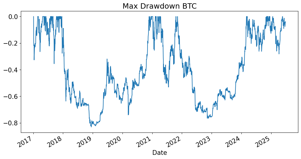
Consider a MDD chart

• For any point in time, it shows how far the strategy is below its max up to that point.

• Whenever it is at 0, the strategy is at a current maximum.

def mdd_timeseries(rets):
    cum_rets = (1 + rets).cumprod()
    rolling_max = cum_rets.cummax()
    drawdown = (cum_rets - rolling_max) / rolling_max
    return drawdown

drawdown = mdd_timeseries(rets)
drawdown[TICK].plot(title=f'Max Drawdown {TICK}');
plt.show()

PLOT_TICKS = ['SPY','UPRO','USO','GLD','BTC','IEF']
n_plots = len(PLOT_TICKS)
n_rows = int(np.ceil(n_plots/2))
fig, ax = plt.subplots(n_rows, 2, figsize=(12, 4*n_rows))
ax = ax.flatten()

for i, tick in enumerate(PLOT_TICKS):
    drawdown[tick].plot(ax=ax[i], title=tick)

plt.suptitle('Maximum Drawdown')
plt.tight_layout()
plt.show()

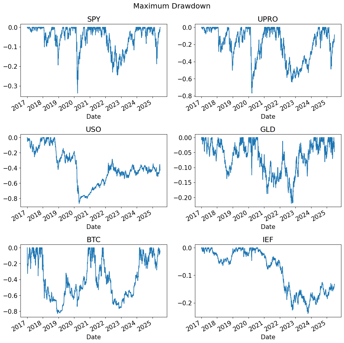
maximumDrawdown(rets).style.format({
    'Skewness': '{:.2f}',
    'Kurtosis': '{:.2f}', 
    'Max Drawdown': '{:.2%}',
    'Peak': lambda x: x.strftime('%Y-%m-%d') if pd.notna(x) else '',
    'Bottom': lambda x: x.strftime('%Y-%m-%d') if pd.notna(x) else '',
    'Recover': lambda x: x.strftime('%Y-%m-%d') if pd.notna(x) else '',
    'Duration (to Recover)': lambda x: f'{x.days:,.0f} days' if pd.notna(x) else ''
})

	Max Drawdown	Peak	Bottom	Recover	Duration (to Recover)
SPY	-33.72%	2020-02-19	2020-03-23	2020-08-10	173 days
VEA	-35.74%	2018-01-26	2020-03-23	2020-11-16	1,025 days
UPRO	-76.82%	2020-02-19	2020-03-23	2021-01-08	324 days
GLD	-22.00%	2020-08-06	2022-09-26	2024-03-04	1,306 days
USO	-86.75%	2018-10-03	2020-04-28
FXE	-26.46%	2018-02-01	2022-09-27
BTC	-83.04%	2017-12-18	2018-12-14	2020-11-30	1,078 days
HYG	-22.03%	2020-02-20	2020-03-23	2020-11-04	258 days
IEF	-23.92%	2020-08-04	2023-10-19
TIP	-14.51%	2021-11-09	2023-10-06
SHV	-0.45%	2020-04-07	2022-06-14	2022-10-07	913 days

Multivariable Risk

All the risk measures above are univariate.

• The measures above for a return \(r\) depend only on functions of the distribution (sample) of \(r\).

We will need to consider multivariable measures.

• As we will see, the risk for a portfolio will require these measures.

Notation

Consider a return on asset \(i\) and \(j\), denoted as \(r_i\) and \(r_j\).

• Note that these superscripts are not exponents but rather identifiers.

Covariance

The covariance is defined as

\[\sigma_{i,j} = \E\left[(r_{i,t}-\mu_i)(r_{j,t}-\mu_j)\right]\]

• A covariance of a variable with itself is the variance.

The sample estimate of the covariance is

\[\hat{\sigma}_{i,j} = \frac{1}{\Ntime}\sum_{t=1}^\Ntime\left(r_{i,t} - \meanest_i\right)\left(r_{j,t} - \meanest_j\right)\]

Covariance Matrix

For \(\Nassets\) assets, it is easier to use matrix notation to write the coviariance \(\sigma_{i,j}\) as the \(i\) row and \(j\) column of the \(\Nassets\times \Nassets\) covariance matrix.

• Note that the diagonal of the matrix is the set of asset variances, \(\sigma_{j,j}=\sigma^2_j\).

Let \(\rmat\) denote the \(\Ntime\times \Nassets\) matrix of sample returns.

• Each of \(\Ntime\) rows is a sample observation (period of time).

• Each of \(\Nassets\) columns is an asset return.

Perhaps somewhat confusingly, it is common to denote this covariance matrix using the capital Greek letter, \(\Sigma\). This looks like a summation sign, but it denotes the \(\Nassets\times \Nassets\) covariance:

\[\covmat = \E\left[(\rvec-\muvec)(\rvec-\muvec)'\right]\]

The sample estimator is the \(\Nassets\times\Nassets\) matrix, $\(\covest = (\rmat-\meanestvec)(\rmat-\meanestvec)'\left(\frac{1}{\Ntime-\Nassets}\right)\)$

where \(\meanest\) denotes the \(\Nassets\times 1\) vector of sample averages:

\[\meanestvec = \rmat'\onevecNt \left(\frac{1}{\Ntime}\right)\]

and where \(\onevecNt\) denotes the \(\Ntime\times 1\) vector of ones.

Technical Note: Properties of the Covariance Matrix

The covariance matrix is

• symmetric: \(\Nassets(\Nassets+1)/2\) unique elements

• positive (semi) definite

Positive definite

• does not mean each element of the matrix, \(\sigma_{i,j}\) is positive

• it means that any combination of the assets will have non-negative variance.

Mathematically, for any \(\Nassets\times 1\) \(w\),

\[w'\covest w\ge 0\]

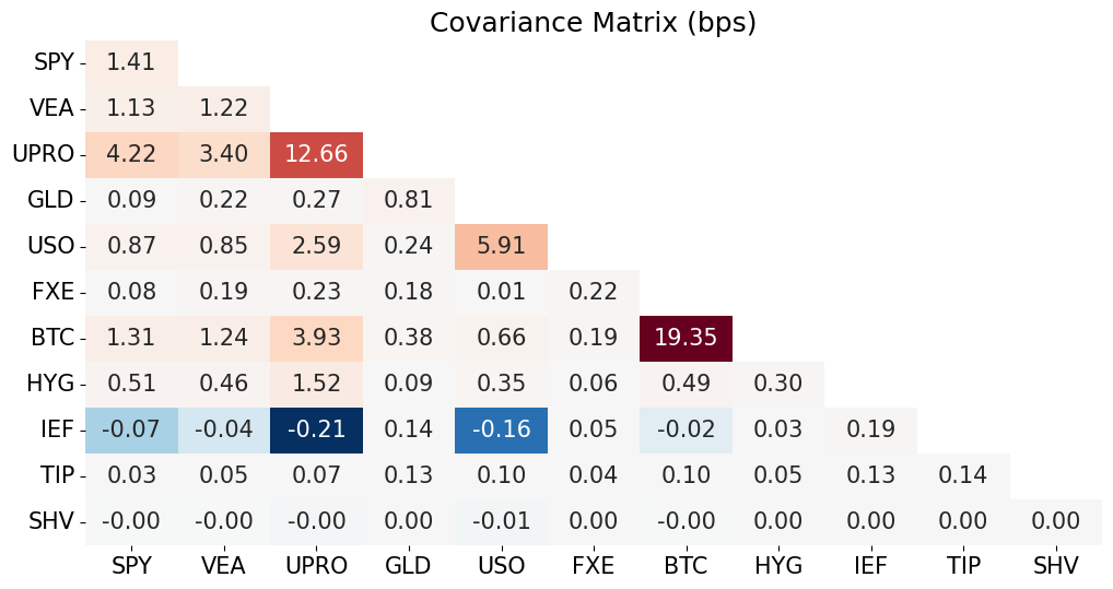
cov_matrix = rets.cov()*100*100

# Set upper triangle to NaN
mask = np.triu(np.ones_like(cov_matrix), k=1)  # Using triu to get upper triangle including diagonal
cov_matrix[mask.astype(bool)] = np.nan

center = 0
vmin = cov_matrix.min().min()
vmax = cov_matrix.max().max()
norm = TwoSlopeNorm(vmin=vmin, vcenter=center, vmax=vmax)
sns.heatmap(cov_matrix, annot=True, fmt='.2f', norm=norm, cmap='RdBu_r', cbar=False)
plt.title('Covariance Matrix (bps)')
plt.show()

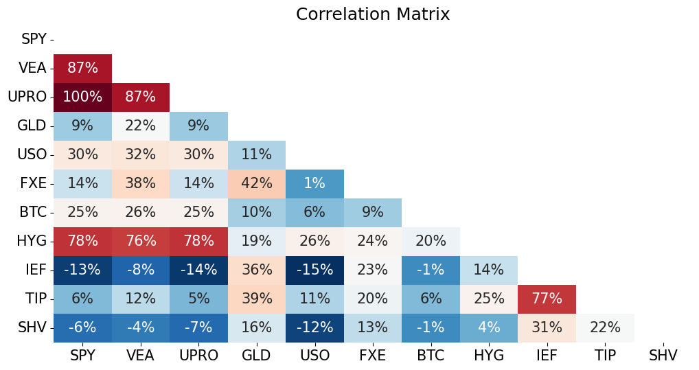
Correlation

The scale of the covariance matrix makes it harder to interpret.

Consider the correlation, which rescales the covariance in a way that is much more useful for interpretation:

• between -1 and 1

• same sign as the covariance

\[\rho_{i,j} = \frac{\sigma_{i,j}}{\sigma_i\sigma_j}\]

Consider the matrix of correlations.

• will be positive semi-definite, as is the covariance matrix.

# Plot correlation matrix
corr_matrix = rets.corr()
plot_triangular_matrix(corr_matrix, title='Correlation Matrix')

Beta

Consider a linear decomposition of \(r_i\) on \(r_j\):

\[r_{i,t} = \alpha + \beta r_{j,t} + \epsilon_t\]

The OLS sample estimator of \(\beta\) is

\[\begin{split}\begin{bmatrix}\hat{\alpha}\\ \hat{\beta}\end{bmatrix} = (\rmat_j'\rmat_j)^{-1}\rmat_j'\rvec_i\end{split}\]

where \(\rmat_j\) denotes the \(N\times 2\) matrix where the first column is a vector of ones and the second column is the vector of sample returns of \(r_{j,t}\) for \(1\le t\le \Ntime\).

Scaled correlation

Equivalently, for a single-variable regression, the beta is simply a scaled correlation:

\[\beta = \frac{\sigma_i}{\sigma_j}\rho_{i,j}\]

The sample estimator is then the product of the sample estimates of these standard deviations and the correlation.

Thus, for bivariate measures,

Covariance, correlation, and beta are just three ways of scaling the relationship

COMP = 'SPY'
birisk = pd.DataFrame(dtype=float, columns=['corr','cov','beta'], index=rets.columns)
birisk['corr'] = rets.corr()[COMP]
birisk['cov'] = rets.cov()[COMP] * FREQ
for sec in rets.columns:
    birisk.loc[sec,'beta'] = LinearRegression().fit(rets[[COMP]],rets[[sec]]).coef_[0]

birisk.columns = [f'{COMP} {col}' for col in birisk.columns]
birisk.style.format({birisk.columns[0]:'{:.1%}',birisk.columns[1]:'{:.1%}',birisk.columns[2]:'{:.2f}'})

	SPY corr	SPY cov	SPY beta
SPY	100.0%	3.6%	1.00
VEA	86.5%	2.9%	0.80
UPRO	99.9%	10.6%	2.99
GLD	8.7%	0.2%	0.07
USO	30.1%	2.2%	0.62
FXE	14.2%	0.2%	0.06
BTC	25.1%	3.3%	0.93
HYG	78.2%	1.3%	0.36
IEF	-13.1%	-0.2%	-0.05
TIP	6.0%	0.1%	0.02
SHV	-6.2%	-0.0%	-0.00

Multivariate Beta

Beta as a rescaled correlation is helpful, but regression betas can be much more.

Consider a multivariate regression:

\[r_{i,t} = \alpha + \beta_j r_{j,t} +\beta_k r_{k,t} + \epsilon_t\]

The OLS sample estimator of \(\beta\) is

\[\begin{split}\begin{bmatrix}\hat{\alpha}\\ \hat{\beta}_j\\ \hat{\beta}_k\end{bmatrix} = (\rmat'\rmat)^{-1}\rmat'\rvec_i\end{split}\]

noting that here \(\rmat\) denotes the matrix with columns of

• ones,

• \(r_{j,t}\)

• \(r_{k,t}\)

That is, each row is an observation, \(t\), and each colmn is a variable, \((1, r_j, r_k)\).

COMPS = ['SPY','VEA']
betas = pd.DataFrame(dtype=float, columns=COMPS, index=rets.columns)
for sec in rets.columns:
    betas.loc[sec] = LinearRegression().fit(rets[COMPS],rets[[sec]]).coef_

betas.join(birisk['SPY beta']).rename(columns={'SPY beta': 'SPY (univariate)'}).style.format('{:.2f}')

	SPY	VEA	SPY (univariate)
SPY	1.00	-0.00	1.00
VEA	0.00	1.00	0.80
UPRO	2.98	0.02	2.99
GLD	-0.32	0.48	0.07
USO	0.22	0.49	0.62
FXE	-0.29	0.43	0.06
BTC	0.43	0.62	0.93
HYG	0.23	0.16	0.36
IEF	-0.09	0.06	-0.05
TIP	-0.06	0.10	0.02
SHV	-0.00	0.00	-0.00

---