TA Review 8

Tobias

Thank you to Tobias for the previous version of this review 🤳

Agenda for today:

1. LTCM

2. Risk Decomposition (feature engineering)

Reading

Optional Reading

John Meriwether is quite famous, and the desk he came from – the fixed income trading desk of Solomon Brother’s – is one of the most notorious desks in finance history. Liar’s Poker by Michael Lewis is a great book about Solomon Brothers.

In 1990-1993, the entirety of Solomon Brother’s lost money, except for their proprietary trading desk, which made so much money that the firm net made money (other business units lost ~20-70m, prop trading made 500m-1.5Bn).

The “LTCM References” page in class.

There are also a lot of Money Stuff articles on some of the trades that LTCM would put on (basis trades).

Required Reading

Some Fun Trades

LTCM’s investment strategy:

• Almost exclusively fixed income and FX, but some options/stock as well.

• Long time horizon (6 months to 2 years)

• Specialized in convergence trades and relative value trades

Let’s walk through some examples:

On the Run/Off the Run bonds

Typically, newly issued US Treasury bonds traded at a higher price (lower yield) than older ones of the same maturity (off the run). So for example, a 30-year bond issued 20 years ago is the same as a 10-year note issued today. But there tends to be a spread between the two, and when this spread widened enough, LTCM would sell the newly-issued 10yr, and buy the older 30-year bond. This is a convergence trade – since you know that eventually the yields of the two have to be the same.

Swap Spread

Interest rate swaps are when one party pays a fixed rate, and the other plays a floating rate (SOFR now, but used to be LIBOR). This lets you bet on the interest rate (or hedge your duration, as you’ll learn next quarter). It also has a “tenor”, which is how long the swap lasts for. So for example, a 30-year swap means that every 6 months for the next 30 years, I’ll pay you whatever SOFR is, and you’ll pay me some fixed amount.

Cashflow wise, this is the same as me lending (receiving interest) at a fixed rate, and borrowing (paying interest) at a floating rate. I can do the same thing with treasury bonds! How? Well, I can repo a treasury bond. This means that I borrow at the repo rate (the interest needed to finance my position), and I can buy the treasury bond with that money. I bought the treasury bond, which means that I’m now lending (receiving interest) at whatever yield that bond is.

Let’s say the swap is quoted at 4.1% and the 2-year bond has a 4% yield. The trade is therefore:

1. Enter a fixed-for-floating-swap, where I pay the fixed rate (4.1%), and receive floating (X%).

2. Repo the 2-year bond at the repo rate (I pay X% - 20bps, and receive the bond’s yield of 4%).

3. Therefore, the only thing that needs to hold for me to make money is that X% - 4.1% > 4% - (X% - 20bps). So you make (SOFR - repo) - (swap - treasury), which is (0.2 - 0.1 = 0.1%)

This is very close to an arbitrage. Equally if the swap was trading below the 2-year, you would do the same thing.

LTCM believed this was very low risk, because:

1. If the swap spread widened, they’d have big mark-to-market gains from the value of the bounds (outweighing the losses on the swap).

2. If the swap spread narrowed, they’d be able to make even more money by just holding it!

Fixed-rate mortages

You can buy government guaranteed mortgages (Fannie/Freddie), at a higher yield than treasuries/interest rate swaps (which are bets purely on government bonds). So, buy the mortgage, hedge your interest rate exposure via a swap and collect the spread. Note that there is some convexity risk here due to pre-payment risk.

Equity relative value

Royal Dutch (listen in Amsterdam) and Shell (listen in London) are the same company. Royal Dutch trades at a premium. So enter into a total return swap where you short Royal Dutch and go long Shell.

Selling Volatility

There are a lot of these structured products, that are really some cash and then some options in a trenchcoat. So for instnace, you might have a bond that pays a 5% coupon, but also gives you upside in the S&P 500. The idea being that if you buy this thing, you’re guaranteed a rate of 5% (the bond part), plus, let’s say 100% of the upside in the S&P if it gains more than 5% that year. This is literally just a bond and a 5% OTM call option. These products will trade a premium to their constituent parts (since they get sold to ~~dentists~~ people).

LTCM recognized that the popularity of these products meant that certain options were priced significantly higher than what historic and projected volatility would be. So if their projections were 10-13% volatility, these might be trading at a 20% volatility. Therefore, you could sell the option, hedge your deltas (exposure to the index), and you can theoretically make a 7% vol point scalp.

(not sure if LTCM) Treasury Basis trade

Treasury futures are actually physically delivered! This means that if you buy a 10yr future and it expires, you will receive a treasury bond. Therefore, the price of a treasury future should just be the current bond that is cheapest-to-deliver (again, foreshadowing for next quarter), and then we can do costs minus benefits.

So if the price of the current bond is 100, and it pays a 5% coupon. Let’s say the repo rate on that bond is 4%. Therefore, the total cost of me financing the bond and holding it for a year is going to be 1% (5% coupon - 4% repo rate). The price of a future on that bond expiring in a year should therefore be 101.

However, treasury futures trade at a premium due to various companies preferring to get rate exposure via futures than via swaps/underlying treasuries. So the future might trade at 102. The trade is therefore buy the bond on repo (receive 5%, pay 4%), and short the treasury future. Then all I need to do is sit and wait and then when the future expires I deliver the bond and close my trade, receiving \(3 (2 from buying the bond at \)100, and selling it at $102, and 1 from carrying the bond for a year, getting a 5% coupon and paying 4% repo on it).

Some Fun Problems

What is the problem with all of these trades? That typically these mispricings are very small. The only way to make a lot of money in them is to lever up in a serious way. On the repo market you can normally get between 50-100x levered (same thing for treasury futures), and swaps are highly levered too.

This is “picking up pennies in front of a bulldozer”, where you are highly levered and are basically scalping a few basis points here and there. The big issue is, to give another quote is that even where trades represent as close to a pure arbitrage as possible, “markets can remain irrational longer than you can remain solvent” (John Maynard Keynes).

If you’re 100x levered and the trade moves against you, or, financing rates, haircuts, etc. change, then you will quickly find yourself getting calls from your clearing house having to unwind the trades. Or, in LTCM’s case being so interconnected across so many institutions that you get bailed out.

Another big problem is cash management. This ties closely to leverage, but because your investor money is scarce, you typically don’t want to put on trades that require an initial cash outlay. Therefore, you want to find trades that use swaps or repos to avoid initial cash requirements that would eat into your returns.

Some Solutions

LTCM did a few things to mitigate mark-to-market losses and financing issues.

First, they were able to get long term repo rates, instead of overnight. You can imagine how much easier the swap-spread trade is if you can repo something for 6 months instead of overnight.

Second, they locked investors into long-term commitments. They weren’t allowed to withdraw money the first year, and then could only withdraw a third of their money in years 2, 3, and 4. This meant that if trades moved against them, they wouldn’t have investors pulling money (remember, their hold time is 6-months to 2-years).

Third, they mitigated counterparty risk via “two-way mark to market”. Normally, if you trade with a big bank, you are the one who gets margin called and has to post collateral. The bank doesn’t need to. LTCM entered in contractual agreements requiring their counterparties also post collateral and mark it to market – and then would exchange money with the counterparty.

Fourth, they had pretty good risk management!? They has both Myron Scholes and Robert Merton as principals, and did typically do a lot of scenario analysis and fairly rigorous risk evaluation.

And then the music stopped

There had been some other losses, but the nail in the coffin was the Russian financial crisis in 1998. The Russian government defaulted on ruble-denominated bonds, which people thought would never happen because they could just print more money to pay for them. This meant that there was a huge “flight to quality” and LTCM was short these bonds and instruments. You’ll recall from the treasury basis trade example that the futures are considered “higher quality” than the underlying bonds, which is why they trade at a premium in the first place! And similarly on the run bonds might be considered higher quality than off the run bonds. So if there is a huge flight to quality, all of your trades move against you at once.

The other thing is is that markets are normally very skittish when selling off, so if rumors spread about you being potentially liquidates, you are all the more likely to get liquidated. From Wikipedia: Victor Haghani, a partner at LTCM, said about this time “it was as if there was someone out there with our exact portfolio,… only it was three times as large as ours, and they were liquidating all at once.”

The Net Interest article on the course page is also very good, and explains how LTCM really functioned more like a bank/service provider than a hedge fund.

Risk Decomposition

The goal here is to understand different aspects of our risks. We might particularly be interested in downside risk, upside risk, etc.

import pandas as pd
import numpy as np
import matplotlib.pyplot as plt
import seaborn as sns
import statsmodels.api as sm

# Have you guys seen Tron?
plt.style.use('dark_background')
plt.rcParams['figure.figsize'] = (8, 5)

def calc_return_metrics(data, as_df=False, adj=12):
    """
    Calculate return metrics for a DataFrame of assets.

    Args:
        data (pd.DataFrame): DataFrame of asset returns.
        as_df (bool, optional): Return a DF or a dict. Defaults to False (return a dict).
        adj (int, optional): Annualization. Defaults to 12.

    Returns:
        Union[dict, DataFrame]: Dict or DataFrame of return metrics.
    """
    summary = dict()
    summary["Annualized Return"] = data.mean() * adj
    summary["Annualized Volatility"] = data.std() * np.sqrt(adj)
    summary["Annualized Sharpe Ratio"] = (
        summary["Annualized Return"] / summary["Annualized Volatility"]
    )
    summary["Annualized Sortino Ratio"] = summary["Annualized Return"] / (
        data[data < 0].std() * np.sqrt(adj)
    )
    return pd.DataFrame(summary, index=data.columns) if as_df else summary


def calc_risk_metrics(data, as_df=False, var=0.05):
    """
    Calculate risk metrics for a DataFrame of assets.

    Args:
        data (pd.DataFrame): DataFrame of asset returns.
        as_df (bool, optional): Return a DF or a dict. Defaults to False.
        adj (int, optional): Annualizatin. Defaults to 12.
        var (float, optional): VaR level. Defaults to 0.05.

    Returns:
        Union[dict, DataFrame]: Dict or DataFrame of risk metrics.
    """
    summary = dict()
    summary["Skewness"] = data.skew()
    summary["Excess Kurtosis"] = data.kurtosis()
    summary[f"VaR ({var})"] = data.quantile(var, axis=0)
    summary[f"CVaR ({var})"] = data[data <= data.quantile(var, axis=0)].mean()
    summary["Min"] = data.min()
    summary["Max"] = data.max()

    wealth_index = 1000 * (1 + data).cumprod()
    previous_peaks = wealth_index.cummax()
    drawdowns = (wealth_index - previous_peaks) / previous_peaks

    summary["Max Drawdown"] = drawdowns.min()

    summary["Bottom"] = drawdowns.idxmin()
    summary["Peak"] = previous_peaks.idxmax()

    recovery_date = []
    for col in wealth_index.columns:
        prev_max = previous_peaks[col][: drawdowns[col].idxmin()].max()
        recovery_wealth = pd.DataFrame([wealth_index[col][drawdowns[col].idxmin() :]]).T
        recovery_date.append(
            recovery_wealth[recovery_wealth[col] >= prev_max].index.min()
        )
    summary["Recovery"] = ["-" if pd.isnull(i) else i for i in recovery_date]

    summary["Duration (days)"] = [
        (i - j).days if i != "-" else "-"
        for i, j in zip(summary["Recovery"], summary["Bottom"])
    ]

    return pd.DataFrame(summary, index=data.columns) if as_df else summary


def calc_performance_metrics(data, adj=12, var=0.05):
    """
    Aggregating function for calculating performance metrics. Returns both
    risk and performance metrics.

    Args:
        data (pd.DataFrame): DataFrame of asset returns.
        adj (int, optional): Annualization. Defaults to 12.
        var (float, optional): VaR level. Defaults to 0.05.

    Returns:
        DataFrame: DataFrame of performance metrics.
    """
    summary = {
        **calc_return_metrics(data=data, adj=adj),
        **calc_risk_metrics(data=data, var=var),
    }
    summary["Calmar Ratio"] = summary["Annualized Return"] / abs(
        summary["Max Drawdown"]
    )
    return pd.DataFrame(summary, index=data.columns)

def calc_univariate_regression(y, X, intercept=True, adj=12):
    """
    Calculate a univariate regression of y on X. Note that both X and y
    need to be one-dimensional.

    Args:
        y : target variable
        X : independent variable
        intercept (bool, optional): Fit the regression with an intercept or not. Defaults to True.
        adj (int, optional): What to adjust the returns by. Defaults to 12.

    Returns:
        DataFrame: Summary of regression results
    """
    X_down = X[y < 0]
    y_down = y[y < 0]
    if intercept:
        X = sm.add_constant(X)
        X_down = sm.add_constant(X_down)

    model = sm.OLS(y, X, missing="drop")
    results = model.fit()

    inter = results.params.iloc[0] if intercept else 0
    beta = results.params.iloc[1] if intercept else results.params.iloc[0]

    summary = dict()

    summary["Alpha"] = inter * adj
    summary["Beta"] = beta

    down_mod = sm.OLS(y_down, X_down, missing="drop").fit()
    summary["Downside Beta"] = down_mod.params.iloc[1] if intercept else down_mod.params.iloc[0]

    summary["R-Squared"] = results.rsquared
    summary["Treynor Ratio"] = (y.mean() / beta) * adj
    summary["Information Ratio"] = (inter / results.resid.std()) * np.sqrt(adj)
    summary["Tracking Error"] = (
        inter / summary["Information Ratio"]
        if intercept
        else results.resid.std() * np.sqrt(adj)
    )
    
    if isinstance(y, pd.Series):
        return pd.DataFrame(summary, index=[y.name])
    else:
        return pd.DataFrame(summary, index=y.columns)


spy = pd.read_excel('gmo_analysis_data.xlsx', sheet_name='total returns', index_col=0, parse_dates=[0])[['SPY']]

As a toy example, lets say that our return is just the market squared (plus some noise). So:

\[ r_i = r_{m}^2 + \epsilon \]

# Make our portfolio follow the -market^2 when market is down, and market when market is up
ex = spy.copy()
ex['Port'] = spy ** 2
# Add noise
ex['Port'] = ex['Port'] + np.random.normal(0, 0.001, size=len(ex))

# Make 2x1 subplots
fig, axes = plt.subplots(ncols=2, nrows=1, figsize=(15, 5))
axes[0].scatter(ex['SPY'], ex['Port'], alpha=0.5)

# Take fit linear regression (quadratic)
sns.regplot(x='SPY', y='Port', data=ex, ax=axes[1], order=2, scatter_kws={'alpha': 0.5}, line_kws={'color': 'red'})

axes[0].set_ylabel('Port')
axes[0].set_xlabel('SPY')

plt.tight_layout()

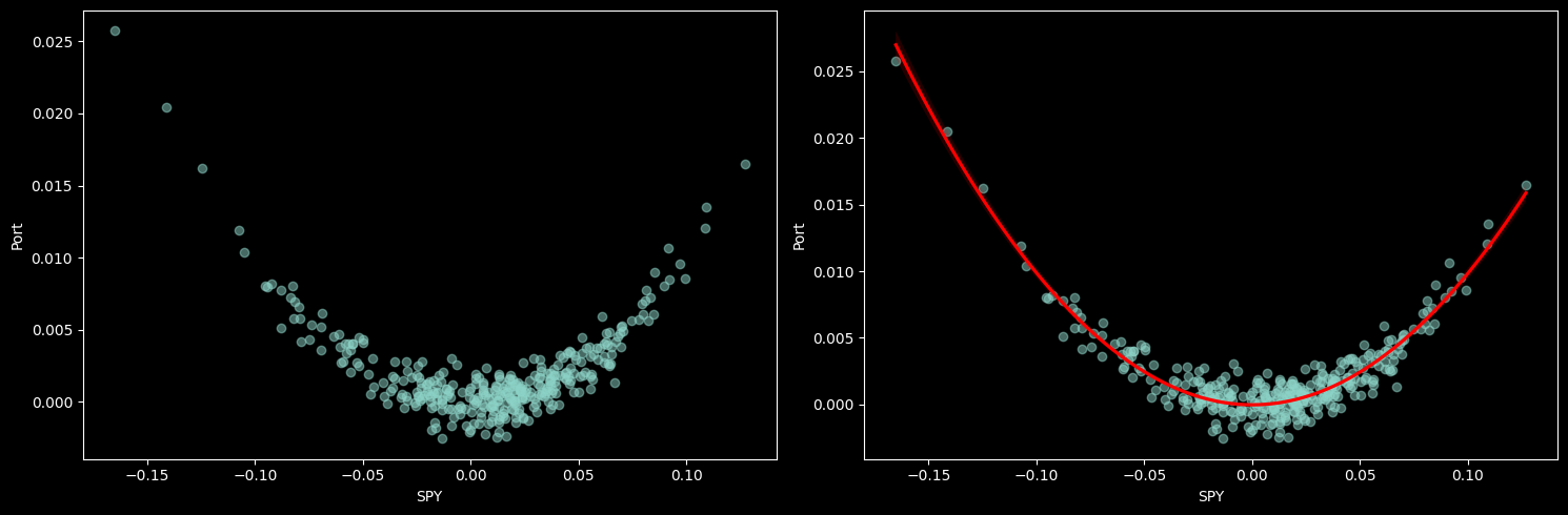
Why might we care both about market beta, and market beta squared?

\[ r_i = \beta_1 r_m + \beta_2 r_m^2 + \epsilon \]

This is ~roughly something like measuring our underlying exposure (delta), and our (realized) volatility exposure (gamma).

What is our payoff is something a little more complicated?

Let’s say we’re long a straddle that is ATM (so 0% returns).

ex['Straddle'] = np.abs(spy.copy())
ex['Straddle'] = ex['Straddle'] + np.random.normal(0, 0.005, size=len(ex))

fig, axes = plt.subplots(ncols=2, nrows=1, figsize=(15, 5))

sns.scatterplot(x='SPY', y='Straddle', data=ex, alpha=0.5, ax=axes[0])
sns.scatterplot(x='SPY', y='Straddle', data=ex[ex['SPY'] < 0], alpha=0.5, ax=axes[1], color='red')
sns.scatterplot(x='SPY', y='Straddle', data=ex[ex['SPY'] > 0], alpha=0.5, ax=axes[1], color='blue');

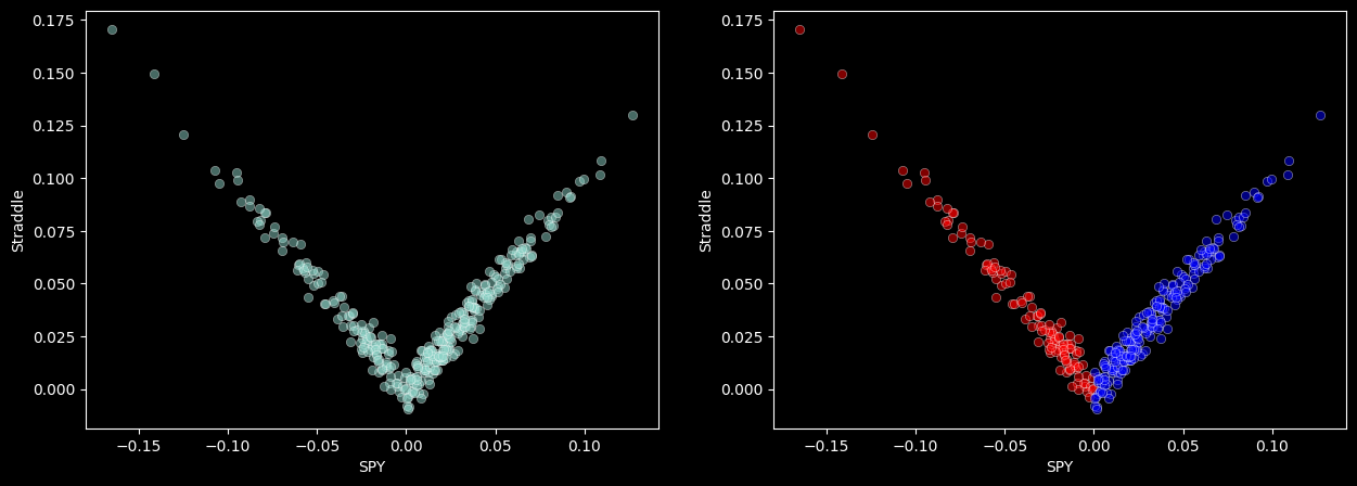
This will obviously have a beta of zero! And maybe some beta squared exposure. However, we can still analyze this using our regression framework, we just need to be smart about how we specify our basis functions (features).

So, lets divide our straddle portfolio into a “put factor” and a “call factor”. So:

\[ r_i = \beta_1 \max(-r_m, 0) + \beta_2 \max(r_m, 0) + \epsilon \]

ex['Put'] = ex['SPY'].copy()
ex.loc[
    ex['SPY'] > 0, 'Put'
] = 0
ex['Put'] = np.abs(ex['Put'])
ex['Call'] = ex['SPY'].copy()

ex.loc[
    ex['SPY'] < 0, 'Call'
] = 0
ex['Call'] = np.abs(ex['Call'])

model = sm.OLS(ex['Straddle'], ex[['Put', 'Call', 'SPY']])
results = model.fit()
results.summary()

OLS Regression Results

Dep. Variable:	Straddle	R-squared (uncentered):	0.987
Model:	OLS	Adj. R-squared (uncentered):	0.987
Method:	Least Squares	F-statistic:	1.298e+04
Date:	Fri, 21 Nov 2025	Prob (F-statistic):	0.00
Time:	18:02:38	Log-Likelihood:	1331.7
No. Observations:	347	AIC:	-2659.
Df Residuals:	345	BIC:	-2652.
Df Model:	2
Covariance Type:	nonrobust

	coef	std err	t	P>|t|	[0.025	0.975]
Put	1.0050	0.007	144.661	0.000	0.991	1.019
Call	1.0022	0.006	158.451	0.000	0.990	1.015
SPY	-0.0028	0.004	-0.665	0.507	-0.011	0.005

Omnibus:	1.158	Durbin-Watson:	1.945
Prob(Omnibus):	0.561	Jarque-Bera (JB):	1.156
Skew:	0.040	Prob(JB):	0.561
Kurtosis:	2.729	Cond. No.	1.29e+16

Notes:
[1] R² is computed without centering (uncentered) since the model does not contain a constant.
[2] Standard Errors assume that the covariance matrix of the errors is correctly specified.
[3] The smallest eigenvalue is 6.39e-33. This might indicate that there are
strong multicollinearity problems or that the design matrix is singular.

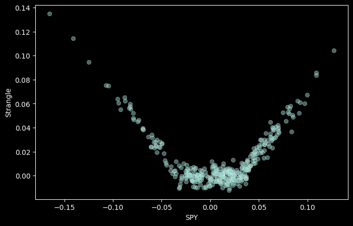
Another example of a non-linear payoff could be being long a strangle (so an OTM put, and an OTM call). Let’s say these are -3% OTM.

ex['Strangle'] = np.maximum(spy - 0.03, 0) + np.maximum(-0.03 - spy, 0)
ex['Strangle'] = ex['Strangle'] + np.random.normal(0, 0.005, size=len(ex))

sns.scatterplot(x='SPY', y='Strangle', data=ex, alpha=0.5);

ex['STG_Put'] = np.maximum(-0.03 - spy, 0)
ex['STG_Call'] = np.maximum(spy - 0.03, 0)
ex['STG_Spy'] = spy
ex['STG_Spy2'] = spy**2

# Fit linear regression
model = sm.OLS(ex['Strangle'], ex[['STG_Put', 'STG_Call', 'STG_Spy', 'STG_Spy2']])
results = model.fit()
results.summary()

OLS Regression Results

Dep. Variable:	Strangle	R-squared (uncentered):	0.962
Model:	OLS	Adj. R-squared (uncentered):	0.962
Method:	Least Squares	F-statistic:	2173.
Date:	Fri, 21 Nov 2025	Prob (F-statistic):	3.86e-242
Time:	18:02:38	Log-Likelihood:	1343.1
No. Observations:	347	AIC:	-2678.
Df Residuals:	343	BIC:	-2663.
Df Model:	4
Covariance Type:	nonrobust

	coef	std err	t	P>|t|	[0.025	0.975]
STG_Put	1.0293	0.075	13.641	0.000	0.881	1.178
STG_Call	1.0411	0.059	17.571	0.000	0.925	1.158
STG_Spy	-0.0064	0.016	-0.407	0.684	-0.037	0.024
STG_Spy2	-0.2160	0.425	-0.508	0.612	-1.052	0.620

Omnibus:	1.265	Durbin-Watson:	2.071
Prob(Omnibus):	0.531	Jarque-Bera (JB):	1.362
Skew:	-0.132	Prob(JB):	0.506
Kurtosis:	2.845	Cond. No.	76.5

Notes:
[1] R² is computed without centering (uncentered) since the model does not contain a constant.
[2] Standard Errors assume that the covariance matrix of the errors is correctly specified.

Why might we care about these “option-like” payoffs? Well, for starters, the put-like factor is basically the same as something like downside beta, where we care about how our portfolio does conditional on the market going down.

Another application of using options is downside protection or PnL smoothing. This is a very popular strategy. The core idea is that most investors tend to be long stock or long the market factor. Therefore, you want to protect your portfolio against large losses, but you don’t want to give up upside (you still want to hold your stock).

One natural way to hedge this would be to buy a put option. This will have a payoff if the market settles below the strike price (or more realistically, will go up in value enough such that we can close our position and realize PnL), and is much easier than just holding less stock, since we still want all of the upside.

The issue with this is that put options are expensive (everyone wants them!). So we could give up some upside in exchange for more insurance, and we can do this by selling a call option.

For example, an equally-struck put option might cost \(10, and the call option might cost \)5. We could therefore buy a put, sell a call, and pay \(5 (down from \)10). So, we can now buy double the amount of put options as we were able to before. Selling a call also has an additional benefit, which is that if we want to protect ourselves, we’re short more deltas.

That trade is what is called a collar/risk reversal/fence.

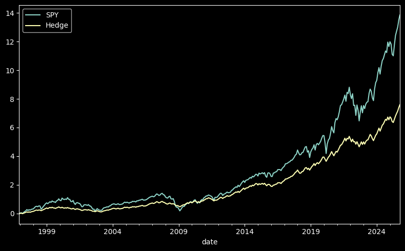
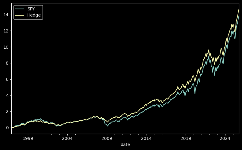
Let’s see how this works in practice. Let’s say we are long SPY, and we want to protect against a 3% monthly drop in SPY. We do this by buying a 3% OTM put, and selling a 3% OTM call.

Maybe the most famous example ever of this here.

ex['Hedge'] = spy.copy() - np.maximum(spy - 0.03, 0) + np.maximum(-0.03 - spy, 0)

# Plot cumulative returns
((1 + ex[['SPY', 'Hedge']]).cumprod() - 1).plot(figsize=(8, 5))
plt.tight_layout()

calc_performance_metrics(
    ex[["SPY", "Hedge"]]
).T

	SPY	Hedge
Annualized Return	0.105537	0.077851
Annualized Volatility	0.153379	0.080651
Annualized Sharpe Ratio	0.688084	0.965287
Annualized Sortino Ratio	0.969596	2.434817
Skewness	-0.558317	-0.466134
Excess Kurtosis	0.789537	-1.374639
VaR (0.05)	-0.074383	-0.03
CVaR (0.05)	-0.096833	-0.03
Min	-0.165187	-0.03
Max	0.126983	0.03
Max Drawdown	-0.507976	-0.236612
Bottom	2009-02-27 00:00:00	2003-02-28 00:00:00
Peak	2025-10-31 00:00:00	2025-10-31 00:00:00
Recovery	2012-03-30 00:00:00	2005-07-29 00:00:00
Duration (days)	1127	882
Calmar Ratio	0.207761	0.329026

calc_univariate_regression(
    y=ex["Hedge"],
    X=ex["SPY"]
).T

	Hedge
Alpha	0.027623
Beta	0.475932
Downside Beta	0.213536
R-Squared	0.819223
Treynor Ratio	0.163576
Information Ratio	0.805534
Tracking Error	0.002858

Note that this improvement even holds if we pick a wider hedge, lets say 5%.

ex['Hedge'] = spy.copy() - np.maximum(spy - 0.05, 0) + np.maximum(-0.05 - spy, 0)

# Plot cumulative returns
((1 + ex[['SPY', 'Hedge']]).cumprod() - 1).plot(figsize=(8, 5))
plt.tight_layout()

calc_performance_metrics(
    ex[["SPY", "Hedge"]]
).T

	SPY	Hedge
Annualized Return	0.105537	0.102068
Annualized Volatility	0.153379	0.113891
Annualized Sharpe Ratio	0.688084	0.89619
Annualized Sortino Ratio	0.969596	1.736196
Skewness	-0.558317	-0.402886
Excess Kurtosis	0.789537	-1.004318
VaR (0.05)	-0.074383	-0.05
CVaR (0.05)	-0.096833	-0.05
Min	-0.165187	-0.05
Max	0.126983	0.05
Max Drawdown	-0.507976	-0.329954
Bottom	2009-02-27 00:00:00	2002-09-30 00:00:00
Peak	2025-10-31 00:00:00	2025-10-31 00:00:00
Recovery	2012-03-30 00:00:00	2005-11-30 00:00:00
Duration (days)	1127	1157
Calmar Ratio	0.207761	0.309339

calc_univariate_regression(
    y=ex["Hedge"],
    X=ex["SPY"]
).T

	Hedge
Alpha	0.027210
Beta	0.709304
Downside Beta	0.466468
R-Squared	0.912469
Treynor Ratio	0.143898
Information Ratio	0.807521
Tracking Error	0.002808

Is this too good to be true? Well, yes. This is one of the reasons why the volatility surface is asymmetric!

def put_skew_vol_smile(strike, atm_strike=100.0, atm_vol=0.20, skew_factor=-0.005, curvature_factor=0.001):
    diff = strike - atm_strike
    implied_vol = atm_vol + (skew_factor * diff) + (curvature_factor * diff**2)
    return implied_vol * 100.0

strikes = np.linspace(90.0, 110.0, 100)

implied_vols = put_skew_vol_smile(strikes, atm_strike=100.0)
const_vols = np.full_like(strikes, 20.0)
plt.plot(strikes, implied_vols, label="Skewed Vol")
plt.plot(strikes, const_vols, label="BS Vol")
plt.legend()
plt.tight_layout()

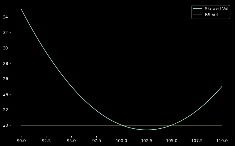
So in reality, this is unfortunately not a free lunch. The puts will trade at a higher implied volatility than the calls, which means that they’ll cost more. The cost of purchasing the puts, even if we sell calls, leads to a drag on our returns.

Let’s say this insurance cost is 2% per year.

ex['Hedge'] = spy.copy() - np.maximum(spy - 0.03, 0) + np.maximum(-0.03 - spy, 0) - 0.02/12

# Plot cumulative returns
((1 + ex[['SPY', 'Hedge']]).cumprod() - 1).plot(figsize=(8, 5))
plt.tight_layout()

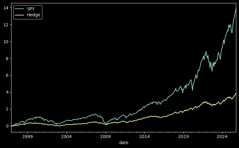
calc_performance_metrics(
    ex[["SPY", "Hedge"]]
).T

	SPY	Hedge
Annualized Return	0.105537	0.057851
Annualized Volatility	0.153379	0.080651
Annualized Sharpe Ratio	0.688084	0.717305
Annualized Sortino Ratio	0.969596	1.636206
Skewness	-0.558317	-0.466134
Excess Kurtosis	0.789537	-1.374639
VaR (0.05)	-0.074383	-0.031667
CVaR (0.05)	-0.096833	-0.031667
Min	-0.165187	-0.031667
Max	0.126983	0.028333
Max Drawdown	-0.507976	-0.283834
Bottom	2009-02-27 00:00:00	2003-02-28 00:00:00
Peak	2025-10-31 00:00:00	2025-10-31 00:00:00
Recovery	2012-03-30 00:00:00	2006-11-30 00:00:00
Duration (days)	1127	1371
Calmar Ratio	0.207761	0.203821

calc_univariate_regression(
    y=ex["Hedge"],
    X=ex["SPY"]
).T

	Hedge
Alpha	0.007623
Beta	0.475932
Downside Beta	0.238137
R-Squared	0.819223
Treynor Ratio	0.121554
Information Ratio	0.222292
Tracking Error	0.002858

What is the point of this HW? We’re trying to engineer features to better explain the returns of the portfolio. This is generally very useful, because it allows us to understand the risks of the portfolio, and then hedge them accordingly, or, “load up” on them synthetically.