import pandas as pd
import numpy as np
from sklearn.linear_model import LinearRegression
from sklearn.decomposition import PCA
import statsmodels.api as sm
import matplotlib.pyplot as plt
import seaborn as sns
import scipy.stats as stats

pd.options.display.float_format = "{:,.4f}".format
plt.style.use('seaborn-v0_8')

from cmds.portfolio import *

# Load S&P 500 individual stock returns
spx_file = '../data/spx_returns_weekly.xlsx'
stock_rets = pd.read_excel(spx_file, 's&p500 rets').set_index('date')
bench_rets = pd.read_excel(spx_file, 'benchmark rets').set_index('date')

# Load sector ETF returns
sector_file = '../data/sector_etf_data.xlsx'
sector_rets = pd.read_excel(sector_file, 'total returns').set_index('date')

print(f"Stock returns shape: {stock_rets.shape}")
print(f"Sector returns shape: {sector_rets.shape}")
print(f"Benchmark returns shape: {bench_rets.shape}")

Stock returns shape: (542, 442)
Sector returns shape: (380, 11)
Benchmark returns shape: (542, 7)

# Align all datasets to common dates
common_dates = stock_rets.index.intersection(sector_rets.index).intersection(bench_rets.index)

# Extract aligned data
stocks = stock_rets.loc[common_dates]
sectors = sector_rets.loc[common_dates]
benchmarks = bench_rets.loc[common_dates]

# Combine sector and benchmark factors (excluding overlapping ETFs)
benchmarks_clean = benchmarks.drop(columns=['SPY','TLT','IYR','BTC'], errors='ignore')
factors = pd.concat([sectors, benchmarks_clean], axis=1)

# Display final dataset information
final_dataset_info = pd.DataFrame({
    'Metric': ['Common Dates', 'Number of Stocks', 'Number of Factors', 'Date Range'],
    'Value': [
        f"{len(common_dates)} observations",
        f"{stocks.shape[1]} stocks", 
        f"{factors.shape[1]} factors",
        f"{common_dates[0].strftime('%Y-%m-%d')} to {common_dates[-1].strftime('%Y-%m-%d')}"
    ]
})
final_dataset_info

	Metric	Value
0	Common Dates	361 observations
1	Number of Stocks	442 stocks
2	Number of Factors	14 factors
3	Date Range	2018-06-29 to 2025-05-23

TICKS = [
    'AAPL',
    'BRK/B',
    'NVDA',
    'TSLA',
    'V',
    'C',
    'LLY',
    'AMZN',
]

# Get OLS metrics for factor decomposition
ols_metrics = get_ols_metrics(factors, stocks, annualization=52)
ols_metrics.loc[TICKS].style.format('{:.1%}',na_rep='-')

	alpha	XLK	XLI	XLF	XLC	XLRE	XLE	XLY	XLB	XLV	XLU	XLP	USO	IEF	GLD	r-squared	Info Ratio
AAPL	7.5%	102.2%	-25.2%	-5.0%	2.0%	8.3%	-1.5%	1.3%	-10.8%	-1.1%	6.5%	36.1%	0.7%	-15.2%	-9.1%	68.3%	46.3%
BRK/B	7.2%	2.2%	5.4%	66.4%	2.9%	-9.4%	3.9%	-18.2%	-0.2%	15.1%	0.3%	18.7%	0.1%	12.5%	-3.3%	74.8%	69.5%
NVDA	22.9%	179.2%	6.7%	-16.7%	-24.0%	-44.5%	-6.2%	48.4%	13.5%	1.9%	9.5%	-57.3%	2.4%	18.5%	8.2%	68.8%	83.6%
TSLA	43.7%	17.8%	-84.6%	-70.9%	-60.4%	-9.9%	16.6%	300.0%	16.3%	-24.2%	29.7%	2.9%	13.0%	-67.8%	2.4%	53.4%	97.1%
V	4.9%	29.5%	-7.5%	42.7%	16.4%	12.6%	-1.3%	-7.2%	-6.4%	8.4%	-9.6%	27.2%	-2.1%	13.4%	-4.8%	62.2%	33.1%
C	-4.6%	0.6%	1.1%	146.3%	9.7%	-6.0%	8.1%	0.8%	-5.0%	-22.6%	3.6%	-21.9%	-1.7%	12.8%	3.9%	81.0%	-28.7%
LLY	29.6%	28.3%	-12.9%	-16.1%	-12.6%	4.3%	16.0%	-19.9%	-20.5%	140.8%	0.3%	-16.3%	-0.6%	12.9%	-3.1%	39.3%	122.0%
AMZN	0.0%	33.2%	-44.3%	0.1%	34.3%	-27.6%	-0.1%	108.0%	-17.8%	10.4%	-7.9%	-5.9%	-1.3%	13.1%	15.7%	67.8%	0.1%

# Perform factor decomposition for each stock
USE_INTERCEPT = True

# Initialize results DataFrames
betas = pd.DataFrame(index=stocks.columns, columns=factors.columns, dtype=float)
residuals = pd.DataFrame(index=stocks.index, columns=stocks.columns, dtype=float)
r_squared = pd.Series(index=stocks.columns, dtype=float)

# Prepare factor matrix (with intercept if needed)
X = factors.copy()
if USE_INTERCEPT:
    X = sm.add_constant(X)
    betas.insert(0, 'alpha', 0)

# Run regressions for each stock
for stock in stocks.columns:
    y = stocks[stock]
    results = sm.OLS(y, X).fit()
    betas.loc[stock] = results.params
    residuals[stock] = results.resid
    r_squared[stock] = results.rsquared

# Display regression summary statistics
regression_summary = pd.DataFrame({
    'value': [
        f"{r_squared.mean():.3f}",
        f"{r_squared.median():.3f}",
        f"{r_squared.min():.3f}",
        f"{r_squared.max():.3f}",
        f"{r_squared.std():.3f}"
    ]
}, index=['Average R2', 'Median R2', 'Min R2', 'Max R2', 'Std R2'])

# Find stocks with min and max R2
min_r2_stock = r_squared.idxmin()
max_r2_stock = r_squared.idxmax()

r2_extremes = pd.DataFrame({
    'Stock': [min_r2_stock, max_r2_stock],
    'R2': [f"{r_squared[min_r2_stock]:.3f}", f"{r_squared[max_r2_stock]:.3f}"]
}, index=['Min R2', 'Max R2'])

display(regression_summary)
display(r2_extremes)

	value
Average R2	0.571
Median R2	0.570
Min R2	0.123
Max R2	0.899
Std R2	0.152

	Stock	R2
Min R2	ERIE	0.123
Max R2	XOM	0.899

---

Dimension Reduction

nPCA = 3

# Compare PCA structure between original returns and residuals
pca_stocks = PCA()
pca_resids = PCA()

pca_stocks.fit(stocks)
pca_resids.fit(residuals)

# Calculate cumulative explained variance for first 5 components
stocks_cum_var = np.cumsum(pca_stocks.explained_variance_ratio_[:nPCA] * 100)
resids_cum_var = np.cumsum(pca_resids.explained_variance_ratio_[:nPCA] * 100)

# Create comparison DataFrame
pca_analysis = pd.DataFrame({
    'Stock Returns Explained (%)': [f"{var:.2f}%" for var in stocks_cum_var],
    'Residuals Explained (%)': [f"{var:.2f}%" for var in resids_cum_var]
}, index=[f'PC{i+1}' for i in range(nPCA)])

pca_analysis

	Stock Returns Explained (%)	Residuals Explained (%)
PC1	40.75%	4.81%
PC2	46.35%	8.26%
PC3	50.41%	11.37%

# Numerical measures of correlation structure
condition_numbers = pd.DataFrame({
    'Dataset': ['Original Returns', 'Residuals', 'Factors'],
    'Condition Number': [
        f"{np.linalg.cond(stocks.corr()):.1e}",
        f"{np.linalg.cond(residuals.corr()):.1e}", 
        f"{np.linalg.cond(factors.corr()):.1e}"
    ],
    'Determinant': [
        f"{np.linalg.det(stocks.corr()):.1e}",
        f"{np.linalg.det(residuals.corr()):.1e}",
        f"{np.linalg.det(factors.corr()):.1e}"
    ],
    'Average Correlation': [
        f"{stocks.corr().abs().mean().mean():.1%}",
        f"{residuals.corr().abs().mean().mean():.1%}",
        f"{factors.corr().abs().mean().mean():.1%}"
    ]
})

condition_numbers

	Dataset	Condition Number	Determinant	Average Correlation
0	Original Returns	1.2e+19	-0.0e+00	39.2%
1	Residuals	4.6e+18	0.0e+00	6.9%
2	Factors	1.0e+02	2.0e-06	50.9%

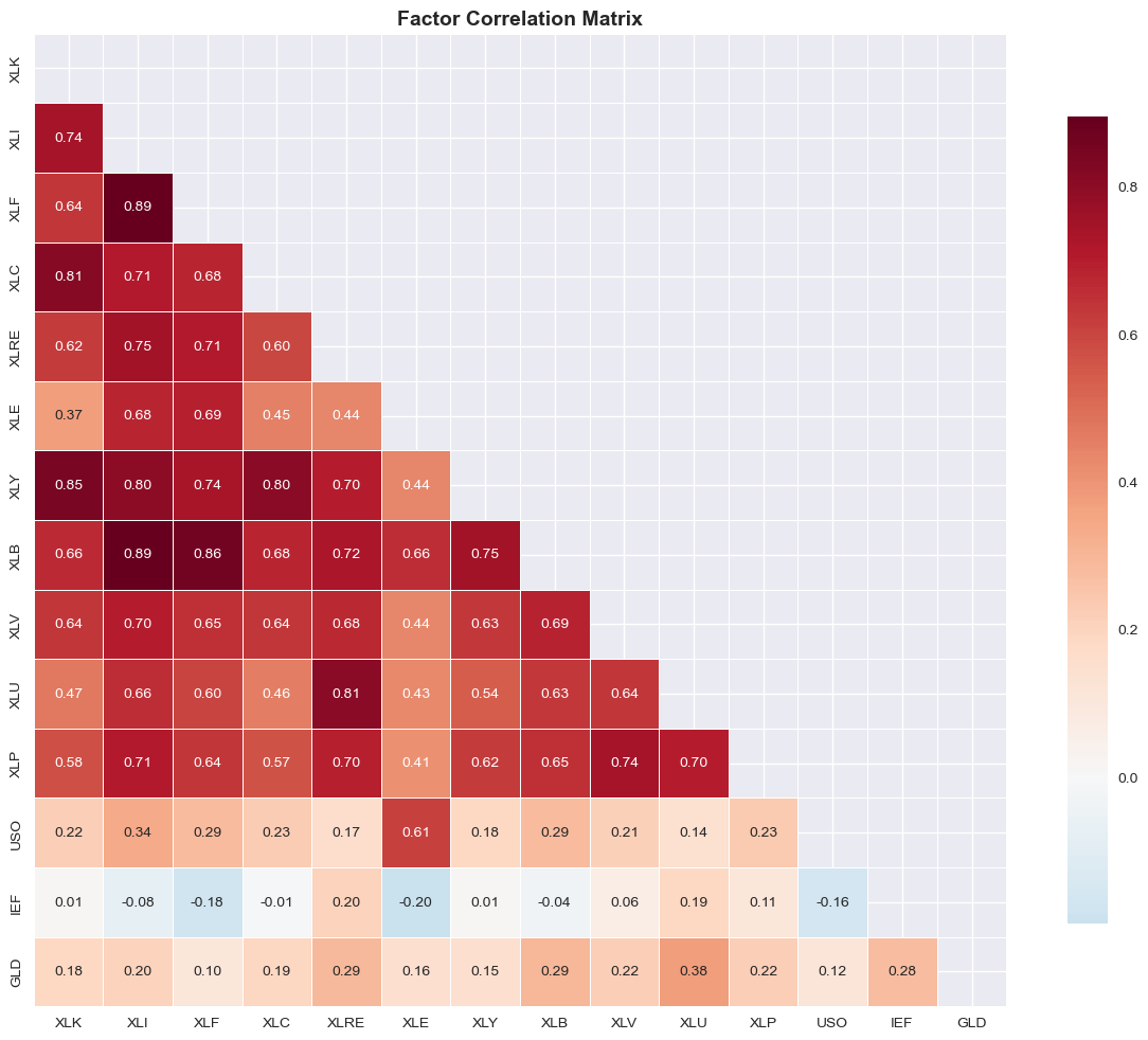
# Factor correlation heatmap
plt.figure(figsize=(12, 10))
corr_matrix = factors.corr()
mask = np.triu(np.ones_like(corr_matrix, dtype=bool))
sns.heatmap(corr_matrix, mask=mask, annot=True, fmt='.2f', cmap='RdBu_r', center=0,
            square=True, linewidths=0.5, cbar_kws={"shrink": 0.8})
plt.title('Factor Correlation Matrix', fontsize=14, fontweight='bold')
plt.tight_layout()
plt.show()

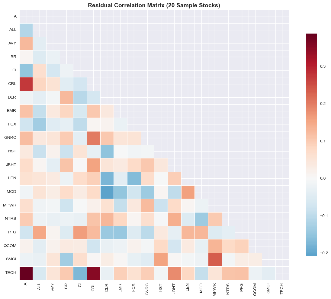
# Residual correlation heatmap (sample of stocks for readability)
# Get 20 stocks spaced evenly through the list
sample_stocks = residuals.columns[::20][:20]  # Take every 20th stock, up to 20 stocks

plt.figure(figsize=(12, 10))
corr_matrix = residuals.loc[:, sample_stocks].corr()
mask = np.triu(np.ones_like(corr_matrix, dtype=bool))
sns.heatmap(corr_matrix, mask=mask, annot=False, fmt='.2f', cmap='RdBu_r', center=0,
            square=True, linewidths=0.5, cbar_kws={"shrink": 0.8})
plt.title('Residual Correlation Matrix (20 Sample Stocks)', fontsize=14, fontweight='bold')
plt.tight_layout()
plt.show()

Reduced Risk

# PRIMARY RESULTS: Key Risk Metrics Comparison

primary_results = pd.DataFrame({
    'Metric': ['Volatility', 'Skewness', 'Kurtosis', 'Average Correlation'],
    'Original Returns': [
        stocks.std().mean(),
        stocks.skew().mean(), 
        stocks.kurtosis().mean(),
        stocks.corr().abs().mean().mean()
    ],
    'Residuals': [
        residuals.std().mean(),
        residuals.skew().mean(),
        residuals.kurtosis().mean(), 
        residuals.corr().abs().mean().mean()
    ],
})

primary_results.set_index('Metric', inplace=True)

primary_results.style.format({
    'Original Returns': '{:.1%}',
    'Residuals': '{:.1%}',
    'Improvement': '{:.4f}'
}, na_rep='-')

primary_results.style.format('{:.1%}',na_rep='-')

	Original Returns	Residuals
Metric
Volatility	4.6%	3.0%
Skewness	0.1%	6.0%
Kurtosis	546.3%	423.0%
Average Correlation	39.2%	6.9%

# Load benchmark returns
benchmark = pd.read_excel(spx_file, sheet_name='benchmark rets')
benchmark.set_index('date', inplace=True)

# Calculate metrics for both stocks and residuals
metrics = {}
for metric, func in [('Volatility', lambda x: x.std()), 
                    ('Skewness', lambda x: x.skew()),
                    ('SPY_Correlation', lambda x: pd.Series({col: x[col].corr(benchmark['SPY']) 
                                                           for col in x.columns}))]:
    # Calculate metric for both stocks and residuals
    stocks_metric = func(stocks)
    residuals_metric = func(residuals)
    
    # Create dataframe with describe statistics for this metric
    metric_df = pd.DataFrame({
        'stocks': stocks_metric.describe(),
        'residuals': residuals_metric.describe()
    })
    metrics[metric] = metric_df

# Combine into multilevel dataframe with metrics as top level
stats_df = pd.concat(metrics, axis=1)
stats_df.style.format('{:.1%}',na_rep='-')

	Volatility		Skewness		SPY_Correlation
	stocks	residuals	stocks	residuals	stocks	residuals
count	44200.0%	44200.0%	44200.0%	44200.0%	44200.0%	44200.0%
mean	4.6%	3.0%	0.1%	6.0%	59.2%	0.1%
std	1.2%	1.0%	47.7%	70.9%	12.2%	0.5%
min	2.5%	1.2%	-241.9%	-617.9%	14.9%	-1.7%
25%	3.7%	2.3%	-26.1%	-22.7%	52.4%	-0.3%
50%	4.3%	2.8%	-1.5%	11.0%	61.1%	0.1%
75%	5.1%	3.4%	23.7%	38.7%	67.6%	0.4%
max	11.1%	9.6%	196.7%	252.4%	82.5%	2.1%

# Summary table of normality improvements across all stocks
all_normality_stats = []

for stock in stocks.columns:
    # Calculate key statistics
    orig_skew = stocks[stock].skew()
    orig_kurt = stocks[stock].kurtosis()
    resid_skew = residuals[stock].skew()
    resid_kurt = residuals[stock].kurtosis()
    
    # Calculate improvement metrics
    skew_improvement = abs(resid_skew) - abs(orig_skew)  # Negative = improvement
    kurt_improvement = abs(resid_kurt) - abs(orig_kurt)  # Negative = improvement
    
    all_normality_stats.append({
        'Stock': stock,
        'Orig_Skew': orig_skew,
        'Resid_Skew': resid_skew,
        'Skew_Change': skew_improvement,
        'Orig_Kurt': orig_kurt,
        'Resid_Kurt': resid_kurt,
        'Kurt_Change': kurt_improvement
    })

normality_summary = pd.DataFrame(all_normality_stats)

# Calculate summary statistics
normality_summary_stats = pd.DataFrame({
    'Metric': [
        'Stocks with Improved Skewness',
        'Stocks with Improved Kurtosis', 
        'Average Skewness Improvement',
        'Average Kurtosis Improvement'
    ],
    'Value': [
        f"{(normality_summary['Skew_Change'] < 0).sum()} / {len(normality_summary)}",
        f"{(normality_summary['Kurt_Change'] < 0).sum()} / {len(normality_summary)}",
        f"{normality_summary['Skew_Change'].mean():.4f}",
        f"{normality_summary['Kurt_Change'].mean():.4f}"
    ]
})
normality_summary_stats

# Show top 10 improvements
top_skew = normality_summary.nsmallest(10, 'Skew_Change')[['Stock', 'Orig_Skew', 'Resid_Skew', 'Skew_Change']]
top_skew

	Stock	Orig_Skew	Resid_Skew	Skew_Change
425	WELL	1.8789	0.1516	-1.7272
417	VTR	1.5470	0.2835	-1.2634
230	KIM	1.9671	0.7868	-1.1803
314	PAYX	-1.0960	0.1423	-0.9537
391	TRGP	-1.1758	-0.2274	-0.9484
327	PM	-1.0759	-0.1405	-0.9354
122	DOC	1.0237	0.1174	-0.9063
126	DTE	0.7894	-0.0039	-0.7856
219	J	-0.8223	-0.0422	-0.7801
234	KMI	-0.7983	-0.0694	-0.7288

# Volatility comparison: Original vs Residuals
vols = pd.DataFrame({
    'Original': stocks.std() * np.sqrt(52),
    'Residuals': residuals.std() * np.sqrt(52)
})

fig, ax = plt.subplots(figsize=(10, 8))
x = vols['Original']
y = vols['Residuals']
ax.scatter(x, y, alpha=0.6, s=50)

# Add 45-degree line
min_val = min(min(x), min(y))
max_val = max(max(x), max(y))
ax.plot([min_val, max_val], [min_val, max_val], 'r--', alpha=0.8, label='45° line')

ax.set_xlabel('Original Volatility (Annualized)', fontsize=12)
ax.set_ylabel('Residual Volatility (Annualized)', fontsize=12)
ax.set_title('Volatility Reduction Through Factor Decomposition', fontsize=14, fontweight='bold')
ax.legend()
ax.grid(True, alpha=0.3)
plt.tight_layout()
plt.show()

print(f"Average volatility reduction: {(1 - vols['Residuals'].mean() / vols['Original'].mean()) * 100:.1f}%")

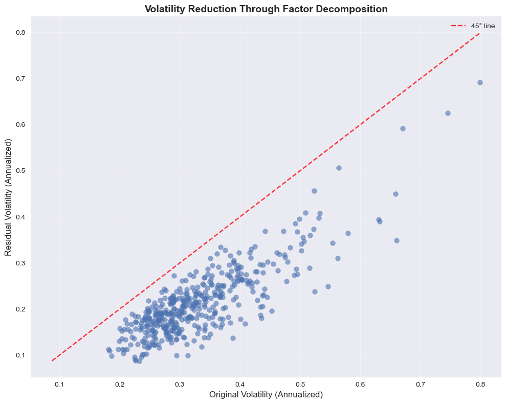
Average volatility reduction: 35.4%

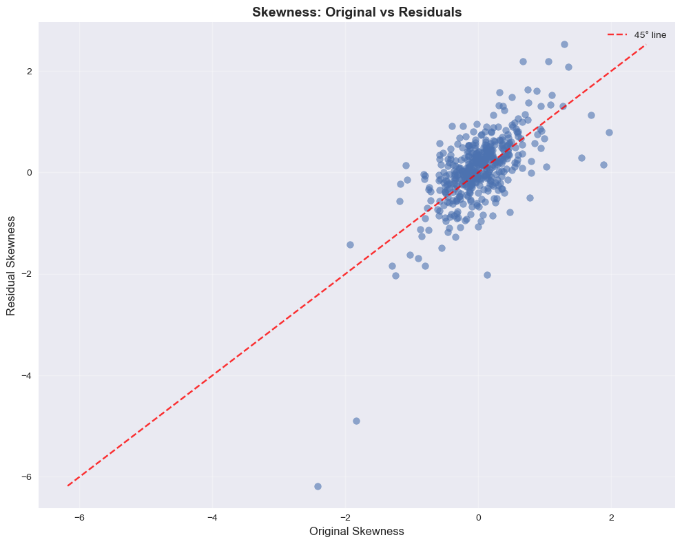
# Skewness comparison: Original vs Residuals
skews = pd.DataFrame({
    'Original': stocks.skew(),
    'Residuals': residuals.skew()
})

fig, ax = plt.subplots(figsize=(10, 8))
x = skews['Original']
y = skews['Residuals']
ax.scatter(x, y, alpha=0.6, s=50)

# Add 45-degree line
min_val = min(min(x), min(y))
max_val = max(max(x), max(y))
ax.plot([min_val, max_val], [min_val, max_val], 'r--', alpha=0.8, label='45° line')

ax.set_xlabel('Original Skewness', fontsize=12)
ax.set_ylabel('Residual Skewness', fontsize=12)
ax.set_title('Skewness: Original vs Residuals', fontsize=14, fontweight='bold')
ax.legend()
ax.grid(True, alpha=0.3)
plt.tight_layout()
plt.show()

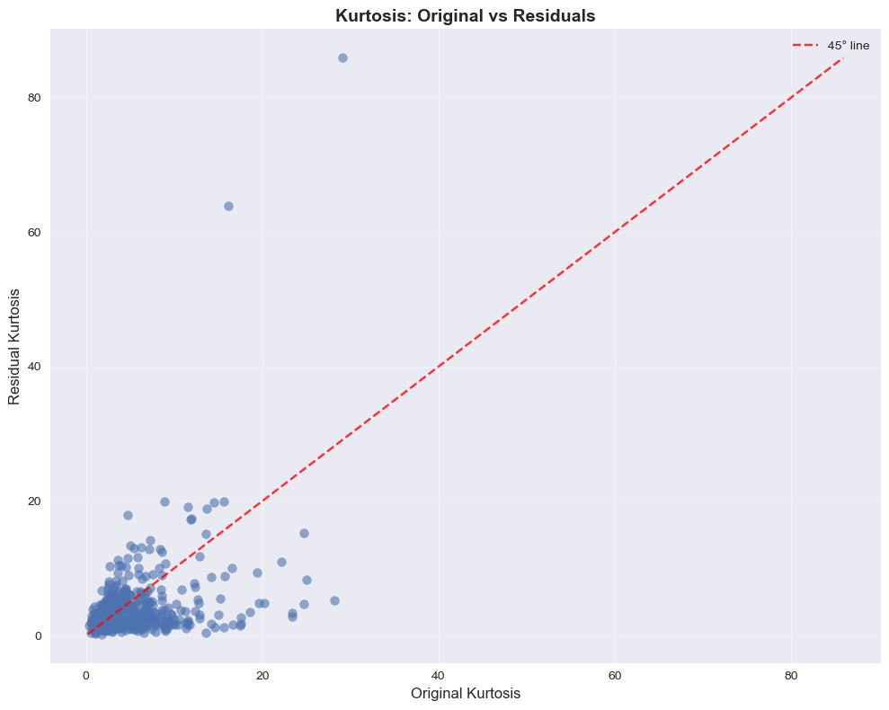
# Kurtosis comparison: Original vs Residuals
kurts = pd.DataFrame({
    'Original': stocks.kurtosis(),
    'Residuals': residuals.kurtosis()
})

fig, ax = plt.subplots(figsize=(10, 8))
x = kurts['Original']
y = kurts['Residuals']
ax.scatter(x, y, alpha=0.6, s=50)

# Add 45-degree line
min_val = min(min(x), min(y))
max_val = max(max(x), max(y))
ax.plot([min_val, max_val], [min_val, max_val], 'r--', alpha=0.8, label='45° line')

ax.set_xlabel('Original Kurtosis', fontsize=12)
ax.set_ylabel('Residual Kurtosis', fontsize=12)
ax.set_title('Kurtosis: Original vs Residuals', fontsize=14, fontweight='bold')
ax.legend()
ax.grid(True, alpha=0.3)
plt.tight_layout()
plt.show()

Normality

# Statistical tests for normality improvement
from scipy.stats import shapiro, jarque_bera, normaltest

# Test normality for a sample of stocks
sample_stocks = ['AAPL', 'MSFT', 'GOOGL', 'AMZN', 'TSLA']
normality_tests = []

for stock in sample_stocks:
    if stock in stocks.columns:
        # Original returns
        orig_stats = {
            'Shapiro-Wilk p-value': shapiro(stocks[stock])[1],
            'Jarque-Bera p-value': jarque_bera(stocks[stock])[1],
            'D\'Agostino p-value': normaltest(stocks[stock])[1]
        }
        
        # Residuals
        resid_stats = {
            'Shapiro-Wilk p-value': shapiro(residuals[stock])[1],
            'Jarque-Bera p-value': jarque_bera(residuals[stock])[1],
            'D\'Agostino p-value': normaltest(residuals[stock])[1]
        }
        
        normality_tests.append({
            'Stock': stock,
            'Original_Shapiro': orig_stats['Shapiro-Wilk p-value'],
            'Residual_Shapiro': resid_stats['Shapiro-Wilk p-value'],
            'Original_JB': orig_stats['Jarque-Bera p-value'],
            'Residual_JB': resid_stats['Jarque-Bera p-value']
        })

normality_df = pd.DataFrame(normality_tests)
normality_df

	Stock	Original_Shapiro	Residual_Shapiro	Original_JB	Residual_JB
0	AAPL	0.0001	0.0113	0.0000	0.0001
1	MSFT	0.0021	0.0000	0.0000	0.0000
2	GOOGL	0.0200	0.0000	0.0114	0.0000
3	AMZN	0.0015	0.0001	0.0002	0.0000
4	TSLA	0.0000	0.0000	0.0000	0.0000

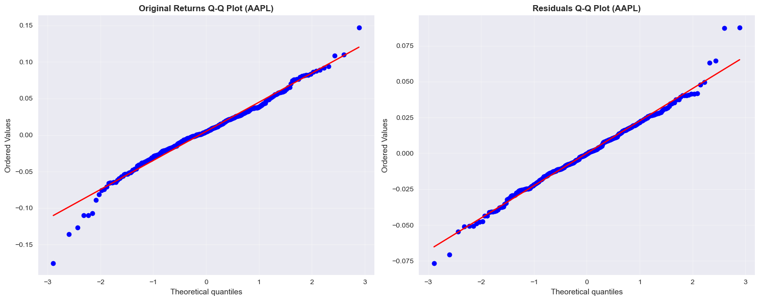
# Q-Q plots for normality assessment
fig, (ax1, ax2) = plt.subplots(1, 2, figsize=(15, 6))

# Original returns Q-Q plot
stats.probplot(stocks['AAPL'], dist="norm", plot=ax1)
ax1.set_title("Original Returns Q-Q Plot (AAPL)", fontweight='bold')
ax1.grid(True, alpha=0.3)

# Residuals Q-Q plot
stats.probplot(residuals['AAPL'], dist="norm", plot=ax2)
ax2.set_title("Residuals Q-Q Plot (AAPL)", fontweight='bold')
ax2.grid(True, alpha=0.3)

plt.tight_layout()
plt.show()

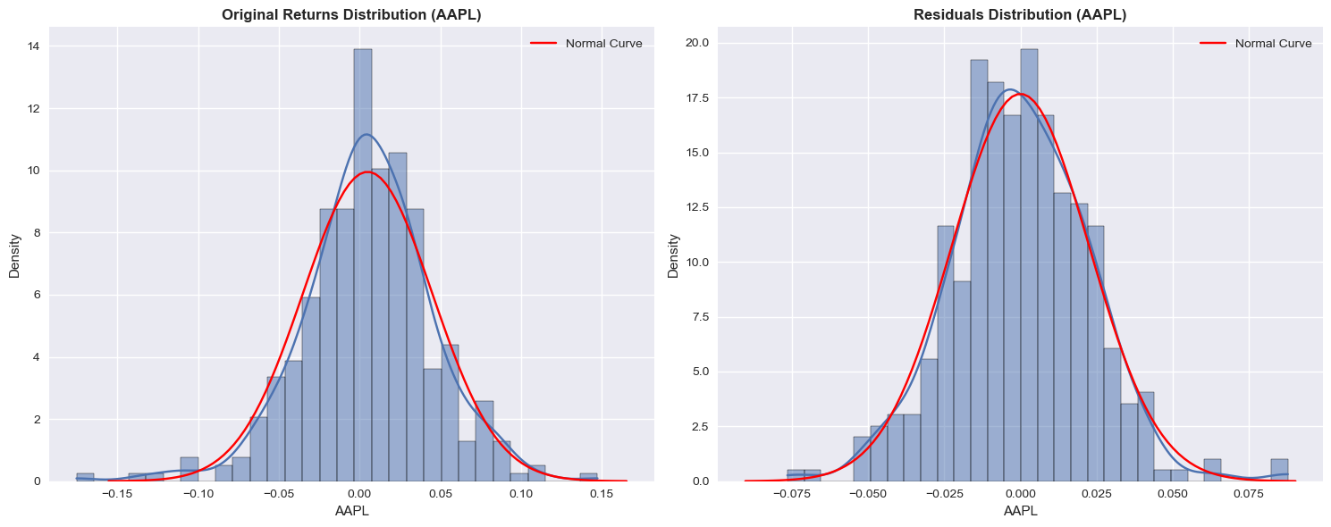
# Distribution comparison: Original vs Residuals
fig, (ax1, ax2) = plt.subplots(1, 2, figsize=(15, 6))

# Original returns distribution
sns.histplot(stocks['AAPL'], kde=True, stat="density", bins=30, ax=ax1)
mean = stocks['AAPL'].mean()
std = stocks['AAPL'].std()
x = np.linspace(mean - 4 * std, mean + 4 * std, 100)
ax1.plot(x, stats.norm.pdf(x, mean, std), label="Normal Curve", color="red")
ax1.set_title("Original Returns Distribution (AAPL)", fontweight='bold')
ax1.legend()

# Residuals distribution
sns.histplot(residuals['AAPL'], kde=True, stat="density", bins=30, ax=ax2)
mean = residuals['AAPL'].mean()
std = residuals['AAPL'].std()
x = np.linspace(mean - 4 * std, mean + 4 * std, 100)
ax2.plot(x, stats.norm.pdf(x, mean, std), label="Normal Curve", color="red")
ax2.set_title("Residuals Distribution (AAPL)", fontweight='bold')
ax2.legend()

plt.tight_layout()
plt.show()

# Statistical tests for normality improvement
from scipy.stats import shapiro, jarque_bera, normaltest

# Test normality for a sample of stocks
sample_stocks = ['AAPL', 'MSFT', 'GOOGL', 'AMZN', 'TSLA']
normality_tests = []

for stock in sample_stocks:
    if stock in stocks.columns:
        # Original returns
        orig_stats = {
            'Shapiro-Wilk p-value': shapiro(stocks[stock])[1],
            'Jarque-Bera p-value': jarque_bera(stocks[stock])[1],
            'D\'Agostino p-value': normaltest(stocks[stock])[1]
        }
        
        # Residuals
        resid_stats = {
            'Shapiro-Wilk p-value': shapiro(residuals[stock])[1],
            'Jarque-Bera p-value': jarque_bera(residuals[stock])[1],
            'D\'Agostino p-value': normaltest(residuals[stock])[1]
        }
        
        normality_tests.append({
            'Stock': stock,
            'Original_Shapiro': orig_stats['Shapiro-Wilk p-value'],
            'Residual_Shapiro': resid_stats['Shapiro-Wilk p-value'],
            'Original_JB': orig_stats['Jarque-Bera p-value'],
            'Residual_JB': resid_stats['Jarque-Bera p-value']
        })

normality_df = pd.DataFrame(normality_tests)
normality_df

	Stock	Original_Shapiro	Residual_Shapiro	Original_JB	Residual_JB
0	AAPL	0.0001	0.0113	0.0000	0.0001
1	MSFT	0.0021	0.0000	0.0000	0.0000
2	GOOGL	0.0200	0.0000	0.0114	0.0000
3	AMZN	0.0015	0.0001	0.0002	0.0000
4	TSLA	0.0000	0.0000	0.0000	0.0000

# Quantify QQ plot improvements with summary statistics
qq_improvements = []

for stock in sample_stocks:
    if stock in stocks.columns:
        # Calculate theoretical quantiles for comparison
        orig_quantiles = np.percentile(stocks[stock], np.linspace(0.1, 99.9, 100))
        resid_quantiles = np.percentile(residuals[stock], np.linspace(0.1, 99.9, 100))
        
        # Theoretical normal quantiles
        theoretical_quantiles = stats.norm.ppf(np.linspace(0.1, 99.9, 100) / 100)
        
        # Calculate deviations from normality
        orig_deviation = np.mean(np.abs(orig_quantiles - theoretical_quantiles))
        resid_deviation = np.mean(np.abs(resid_quantiles - theoretical_quantiles))
        
        qq_improvements.append({
            'Stock': stock,
            'Original_Deviation': orig_deviation,
            'Residual_Deviation': resid_deviation,
            'Improvement_%': (1 - resid_deviation / orig_deviation) * 100
        })

qq_df = pd.DataFrame(qq_improvements)
qq_df

	Stock	Original_Deviation	Residual_Deviation	Improvement_%
0	AAPL	0.7883	0.8010	-1.6212
1	MSFT	0.7920	0.8061	-1.7901
2	GOOGL	0.7873	0.8012	-1.7632
3	AMZN	0.7852	0.7997	-1.8535
4	TSLA	0.7485	0.7736	-3.3470

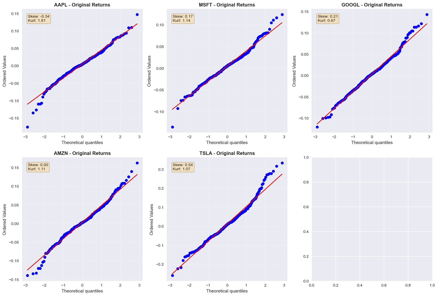
# Visual comparison of normality improvements
fig, axes = plt.subplots(2, 3, figsize=(18, 12))
axes = axes.flatten()

for i, stock in enumerate(sample_stocks[:6]):
    if stock in stocks.columns and i < 6:
        ax = axes[i]
        
        # Create side-by-side QQ plots
        stats.probplot(stocks[stock], dist="norm", plot=ax)
        ax.set_title(f'{stock} - Original Returns', fontweight='bold')
        ax.grid(True, alpha=0.3)
        
        # Add statistics as text
        orig_skew = stocks[stock].skew()
        orig_kurt = stocks[stock].kurtosis()
        ax.text(0.05, 0.95, f'Skew: {orig_skew:.2f}\nKurt: {orig_kurt:.2f}', 
                transform=ax.transAxes, verticalalignment='top',
                bbox=dict(boxstyle='round', facecolor='wheat', alpha=0.8))

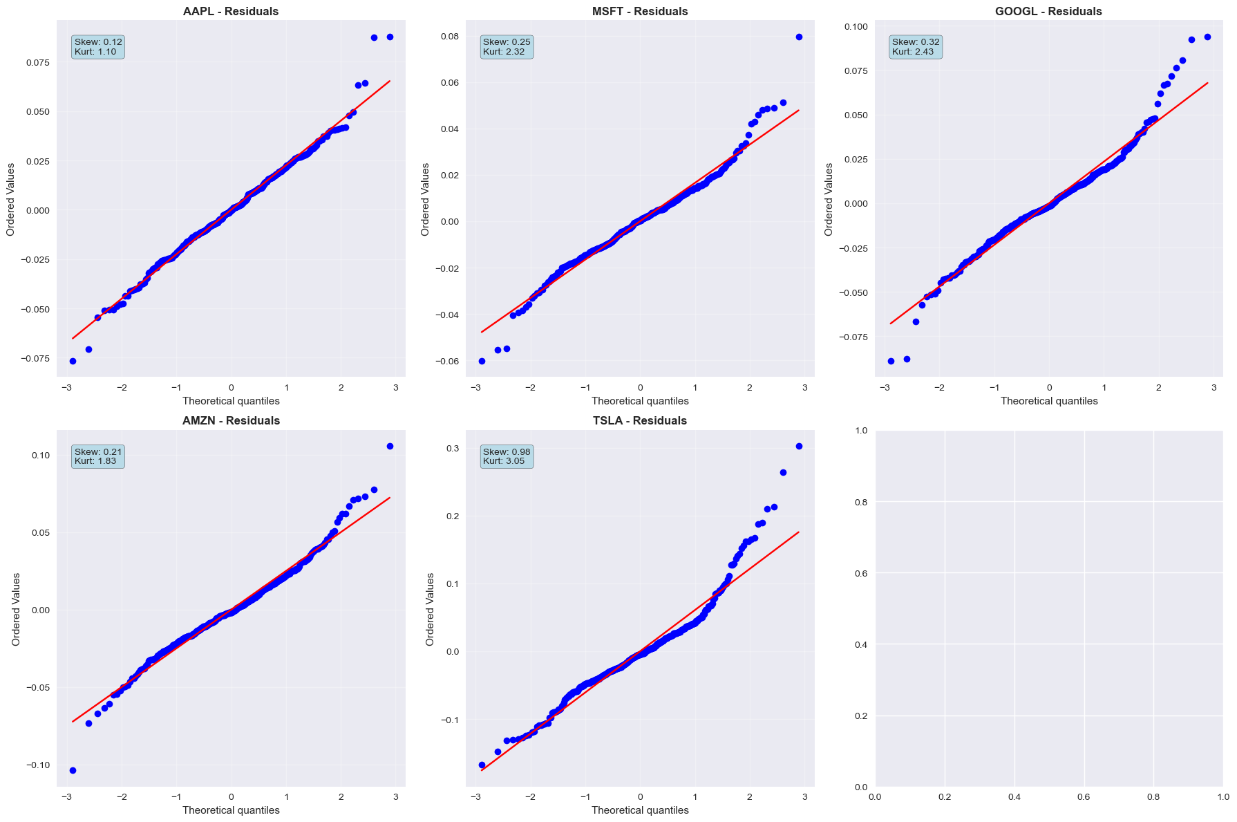
# Add residuals QQ plots
fig2, axes2 = plt.subplots(2, 3, figsize=(18, 12))
axes2 = axes2.flatten()

for i, stock in enumerate(sample_stocks[:6]):
    if stock in residuals.columns and i < 6:
        ax = axes2[i]
        
        stats.probplot(residuals[stock], dist="norm", plot=ax)
        ax.set_title(f'{stock} - Residuals', fontweight='bold')
        ax.grid(True, alpha=0.3)
        
        # Add statistics as text
        resid_skew = residuals[stock].skew()
        resid_kurt = residuals[stock].kurtosis()
        ax.text(0.05, 0.95, f'Skew: {resid_skew:.2f}\nKurt: {resid_kurt:.2f}', 
                transform=ax.transAxes, verticalalignment='top',
                bbox=dict(boxstyle='round', facecolor='lightblue', alpha=0.8))

plt.tight_layout()
plt.show()