Optimizing Risk and Return#
Performance Measures#
We have discussed various measures of risk.
Of course, we care about return as well as risk.
We might be willing to take more risk for more return.
Below are measures of return and the risk-return tradeoff.
Excess Returns#
Many performance measures, as well as optimizations, will focus on excess returns. That is, the return on the portfolio /security beyond the risk-free rate.
We use tilde notation for excess returns to avoid writing the risk-free rate everywhere. That is,
Mean Return#
Mean (total or excess) return is the most utilized measure of ex-ante reward in an investment.
Most allocation and risk measures will consider mean return against some form of risk.
If we are focusing on USD, not returns, then we might label this as expected value (EV).
Alpha#
The second widely used measure of “reward” is alpha.
Consider a regression of the portfolio (or security) return against a benchmark, in this case, SPY.
Note that we might be interested in a decomposition against several factors, \(\boldsymbol{x}_t\).
We will have more to say about these decompositions.
Alpha as a measure of performance#
Alpha is measuring the mean return of the portfolio (security) beyond what can be explained by the regressors.
We may have a high mean return simply due to loading up on lots of factor risk.
Consider UPRO, the 3x levered S&P500 ETF.
For this reason, alpha is widely cited in judging (hedge / mutual) fund performance.
Did the fund earn high mean returns beyond what we would expect from their broad factor exposures?
In a sense, did we get any mean return beyond what we would have received from holding an (few?) index funds?
import pandas as pd
import numpy as np
import datetime

import matplotlib.pyplot as plt
%matplotlib inline
plt.rcParams['figure.figsize'] = (10,5)
plt.rcParams['font.size'] = 13
plt.rcParams['legend.fontsize'] = 13

from matplotlib.ticker import (MultipleLocator,
                               FormatStrFormatter,
                               AutoMinorLocator)

from sklearn.linear_model import LinearRegression
from cmds.portfolio import *
from cmds.risk import *
LOADFILE = '../data/risk_etf_data.xlsx'
info = pd.read_excel(LOADFILE,sheet_name='descriptions').set_index('ticker')
rets = pd.read_excel(LOADFILE,sheet_name='total returns').set_index('Date')
prices = pd.read_excel(LOADFILE,sheet_name='prices').set_index('Date')

retsx = rets.sub(rets['SHV'],axis=0)
FREQ = 252
doEXCESS = True
COMP = 'SPY'


if doEXCESS:
    data = retsx
else:
    data = rets


regs = pd.DataFrame(dtype=float, columns=['mean','alpha','beta'], index=rets.columns)
for sec in rets.columns:
    est = LinearRegression().fit(data[[COMP]],data[[sec]])
    regs.loc[sec,'alpha'] = est.intercept_
    regs.loc[sec,'beta'] = est.coef_[0]

regs['mean'] = retsx.mean()
regs[['mean','alpha']] *= FREQ
regs.style.format({'mean':'{:.2%}','alpha':'{:.2%}','beta':'{:.2f}'})
| mean | alpha | beta | |
|---|---|---|---|
| SPY | 13.13% | 0.00% | 1.00 |
| VEA | 7.54% | -3.01% | 0.80 |
| UPRO | 36.69% | -2.60% | 2.99 |
| GLD | 10.72% | 9.87% | 0.06 |
| USO | 2.86% | -5.28% | 0.62 |
| FXE | -0.56% | -1.29% | 0.06 |
| BTC | 77.14% | 64.93% | 0.93 |
| HYG | 2.49% | -2.24% | 0.36 |
| IEF | -0.90% | -0.26% | -0.05 |
| TIP | 0.60% | 0.35% | 0.02 |
| SHV | 0.00% | 0.00% | -0.00 |
Treynor#
The Treynor ratio is the tradeoff between mean excess return and beta.
This is mostly used with equities, where the beta is with regard to a broad equity benchmark, like SPY.
Information Ratio#
The Information Ratio is the tradeoff between alpha and unexplained volatility.
A regression of \(\rx_{i,t}\) onto a factor (benchmark) \(x_t\) reveals the unexplained…
mean: \(\alpha\)
movements: \(\epsilon\)
volatility: \(\sigma_\epsilon\) as well as the explained portion, \(\beta x\).
The Information Ratio is thus the Sharpe ratio of the unexplained portion of the decomposition, \(\alpha\) versus \(\epsilon\).
keyX = 'SPY'
tab = pd.concat([performanceMetrics(retsx,annualization=FREQ)['Sharpe'],get_ols_metrics(retsx[keyX],retsx,annualization=FREQ)[['Info Ratio','Treynor Ratio']]],axis=1)
tab.fillna(np.nan,inplace=True)
tab.style.format({'alpha':'{:.2%}','Sharpe':'{:.2%}','r-squared':'{:.2%}','Treynor Ratio':'{:.2%}','Info Ratio':'{:.2%}'})
/var/folders/zx/3v_qt0957xzg3nqtnkv007d00000gn/T/ipykernel_27595/425171981.py:3: FutureWarning: Downcasting object dtype arrays on .fillna, .ffill, .bfill is deprecated and will change in a future version. Call result.infer_objects(copy=False) instead. To opt-in to the future behavior, set `pd.set_option('future.no_silent_downcasting', True)`
  tab.fillna(np.nan,inplace=True)
| Sharpe | Info Ratio | Treynor Ratio | |
|---|---|---|---|
| SPY | 69.60% | nan% | 13.13% |
| VEA | 43.06% | -34.28% | 9.39% |
| UPRO | 64.92% | -97.88% | 12.26% |
| GLD | 75.32% | 69.59% | 165.45% |
| USO | 7.40% | -14.35% | 4.61% |
| FXE | -7.63% | -17.77% | -10.06% |
| BTC | 110.45% | 96.05% | 83.00% |
| HYG | 28.72% | -41.50% | 6.92% |
| IEF | -13.23% | -3.91% | 18.58% |
| TIP | 10.08% | 5.89% | 31.51% |
| SHV | nan% | nan% | nan% |
Diversification#
Subadditivity#
Variance of a Portfolio#
Consider a portfolio of \(\Nsec\) risky securities.
return volatility is \(\sigma_i\)
return covariance is \(\sigma_{i,j}\)
weight in security \(i\) is given by \(\wt_i\), with $\(\sum_{i=1}^\Nsec \wt_i = 1\)$
Then
Suppose we have an equally-weighted portfolio, \(w_i=\frac{1}{\Nsec}\) for all \(i\).
Then it is easy to shwo that
As the portfolio increases the number of securities, \(\Nsec\to\infty\), we have
Individual variances do not have much impact on portfolio variance!#
Technical Points#
Equal weights?#
A similar result would hold even if we didn’t assume equal weights, so long as no single weight held a large share in the portfolio.
Simplified formula#
For pedagogy, assume all \(\Nsec\) volatilites are equal and that all pairwise correlations are \(\rho\). Then we would have
which makes the point that as \(\Nsec\) grows, the portfolio variance is a fraction of the common variance, where the fraction is given by \(\rho\).
This illustrates the idea of the total risk \(\sigma^2\) having two components
systematic, \(\rho\sigma^2\)
idiosyncratic
In more general settings, we see a similar phenomenon, that total risk decreases due to the subadditivity.
Stand-alone vs Marginal Risk#
More broadly, the risk measure of a single asset (standalone risk) is very different from its contribution of risk to a portfolio.
We saw this above for variance, but it is true for any subadditive risk measure.
Consider normal VaR, (recalling that general VaR is not subadditive.)
Normal Value-at-risk#
That is, the marginal VaR to portfolio \(p\) with \(\Nsec\) assets is a function of the covariances, not its own volatility.
Thus, marginal (normal) VaR is quite different from standalone (normal VaR).
Mean Additivity#
We have discussed subadditivity and diversification for risk. What about for mean return (reward)?
The mean is a linear function!
Thus, it is additive, not subadditive.
With means, the “whole” is exactly equal to the “sum of its parts.”
Thus, diversification reduces risk while leaving mean return intact!#
This is the reason that diversification is seen as a free lunch.
Example: Mean vs Volatility for Two Assets#
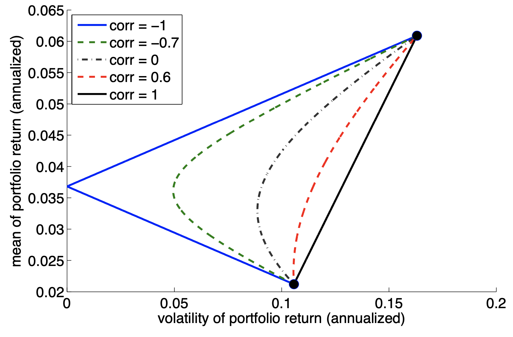
Mean-Variance Optimization#
For two assets, we saw diversification means
subadditive risk
additive mean
This holds for a portfolio of \(\Nsec\) risky securities.
Consider the mean variance optimization. Equivalently,
mean-volatility optimization
Sharpe Ratio optimization
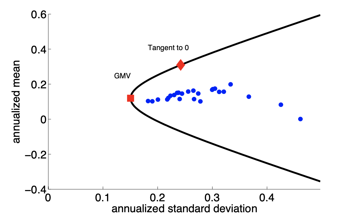
Figures on the Diversification#
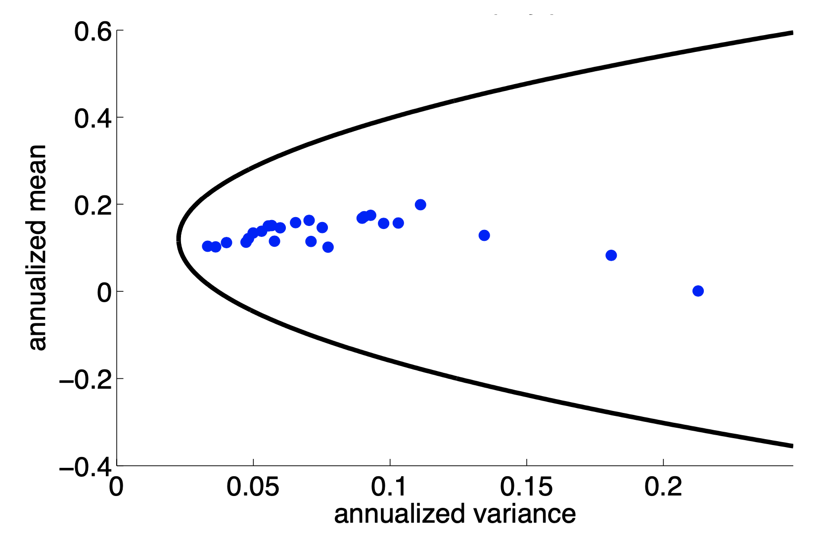
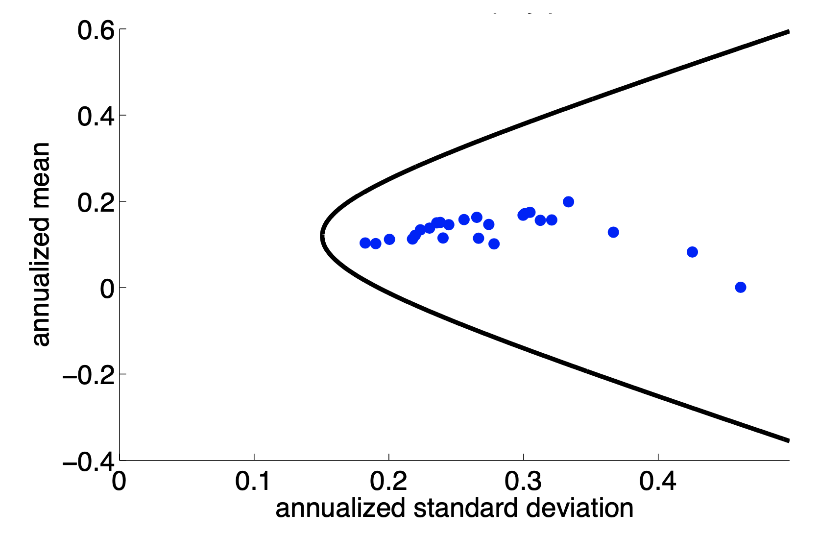
Preliminaries#
Consider a problem of
\(\Nsec\) risky assets
cash (or some other risk-free asset)
frictionless markets–long short any amount
weights on risky assets do not need to equal 1, as cash can be long/short $\(\wtvec'\boldsymbol{1} \ne 1\)$
We will consider excess returns
makes the math a little simpler
good assumption if we have ability to leverage with cash
Recall that covariance
matrix of \(\Nsec\) securities is \(\covmat\)
of the total chosen portfolio is $\(\sigma^2_p = \wtvec'\covmat\wtvec\)$
Optimization#
Background#
Here we use a few simple results from calculus and optimization. For a refresher, see this link.
Objective#
The objective is to minimize portfolio variance.
The Constraint#
The constraint is to achieve a mean return target:
Note#
We have not added constraints on…
sum of weights
short positions
individual position sizes
Duality#
This optimization is of a special type such that its dual would give the same solution set. Namely,
Objective: maximize return
Constraint: achieve a set variance
Technical Point#
This is a linear program.
Setting up the Problem#
A mean-variance portfolio is a vector, \(\wtvec^*\) which solves the following constrained optimization for some mean excess return target \(m\).
What makes for an easy optimization#
Optimizations are often intractable.
This optimization is easy.
Why?
Technical Point:#
Given the simplicity of this optimization, we can solve it analytically, with an explicit solution:
Set up the Lagrangian with just one constraint.
The FOC is sufficient given the convexity of the problem.
Finally, substitute the Lagrange multiplier using the constraint.
The solution#
where \(\delta_m\) is simply a scaling constant to ensure we hit the mean of \(m\).
Note that#
All solutions are just a rescaling of \(\covmat^{-1}\muxvec\)
In fact, there is a name for this baseline: the tangency portfolio.
where \(\delta_\tan\) is a number that ensures \(\wtvec^{\tan}\) sums to one.
We are not insisting all solutions add to one. But it is useful to highlight this special solution that does add to one.
Technical Point#
The forumulas for the scalings look tedious but are easy to calculate.
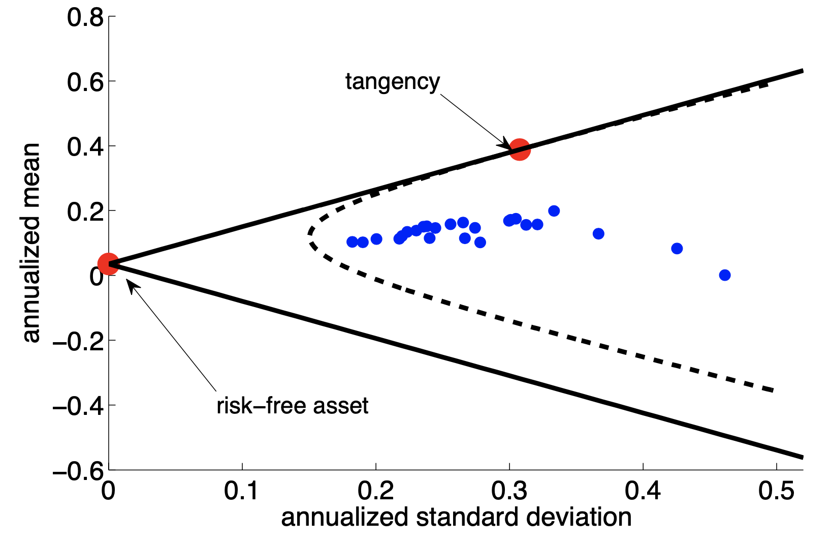
Two Fund Separation#
This is known as two-fund separation.
Every investor should invest (long or short) cash and (long or short) the tangency portfolio.
Variation in investor risk will lead to different solutions, but even with \(\Nsec\) assets, everyone holds the exact same bundle, (the tangency portfolio,) in different sizes.
Additional Constraints#
No cash (weights add to one)#
We could optimize the space of total (not excess) returns for a situatoin where there is no cash asset.
Then, the weights need to add to one.
This would introduce a second constraint to the optimization above:
Still an easy optimization.
Adds a second dimension to the solution.
Thus, all investors hold a mix of two risky bundles (tangency and minimum variance) instead of tangency and cash.
One could see this solution as deriving “synthetic” cash (to the best of its ability) and then getting back to an anologous solution.
Position Constraints#
We may wish to constrain individual security weights, \(\wt_i\).
No short positions, \(\wt_i\ge 0\)
Mandate to hold at least/most, \(\wt_i\ge c\), \(\wt_j\le c\).
These constraints will cause us to lose an explicit solution formula.
Why?
Still, the optimization problem is easy numerically.
Why?
See the other notebook for an illustration of these constraints.
Beyond Variance#
These optimizations have been mean-variance.
We have discussed that there are many other risk measures we may want to consider.
What would be needed to optimize…
mean-volatility
mean-Normal VaR
information ratio
mean-to-VaR
mean-to-CVaR
Appendix#
One Weird Trick Your Statistician Will HATE#
Mean-variance optimization is actually a linear regression!
Look back at the formula for the tangency weights
\(\covmat\) is like \(X'X\)
\(\muxvec\) is like \(X'\boldsymbol{1}\)
Takes some tedious algebra, but can be shown that the tangency weights, (solving the MV problem) are obtained by the following, (weird!) regression:
Why do we care? The MV formula is easy to compute?
We can apply the many techniques and tricks of regression to portfolio optimization.
Extra Notebook#
See the appendix if interested in more on this.