Solution - Reversals

Thanks to Anand Nakhate

1. Investigate Reversals

Data

Find monthly data on the long-term reversal factor.

• LT Reversal (excess returns)

• deciles (total returns)

1.1.

Report summary statistics for the reversal factor.

1.2.

Report the summary statistics for the low and high decile from deciles (total returns).

Do you see evidence of differential performance?

Plot the cumulative return of each.

1.3.

Does your answer to 1.2 change if we focus just on data since Jan 2001?

1.4.

Staying with the later subsample, do you see evidence that the results are significantly impacted by small stocks?

Use size_sorts (total returns) to compare BIG LoPRIOR to BIG HiPRIOR.

---

1.

KEY = 'REV'
TAG_LONG = 'Lo'
TAG_SHORT = 'Hi'

YR_CUTOFF = '2001'
YR_LAST_PRIOR_CUTOFF = '2000'

periods = [['1927', '2025'], ['1927', YR_LAST_PRIOR_CUTOFF], [YR_CUTOFF, '2025']]

FILE_PATH = '../data/reversal_data.xlsx'

SHEET_factors = 'FF factors (excess returns)'
SHEET_momentum = 'LT Reversal (excess returns)'
SHEET_deciles = 'deciles (total returns)'
SHEET_size_sorts = 'size_sorts (total returns)'
SHEET_rf = 'risk-free rate'

ANN_SCALE = 12

from functools import partial
import pandas as pd
import numpy as np
import seaborn as sns
import statsmodels.api as sm
import matplotlib.pyplot as plt

plt.style.use('ggplot')

import sys
if '../cmds/' not in sys.path:
    sys.path.append('../cmds/')
from portfolio_management_helper import *

import warnings
warnings.filterwarnings("ignore")

raw_data = pd.read_excel(FILE_PATH,sheet_name = None)
ff_factors = raw_data[SHEET_factors].set_index('Date')
momentum = raw_data[SHEET_momentum].set_index('Date')
mom_deciles = raw_data[SHEET_deciles].set_index('Date')
tercile_port = raw_data[SHEET_size_sorts].set_index('Date')
rf = raw_data[SHEET_rf].set_index('Date')

ff_factors[KEY] = momentum[KEY]

1.1.

summary_col_names = ['Annualized Mean','Annualized Vol','Annualized Sharpe','Skewness']
res = []
for period in periods:
    temp = momentum.loc[period[0]:period[1]]
    temp_ff = ff_factors.loc[period[0]:period[1]]
    summary = calc_summary_statistics(temp, annual_factor=ANN_SCALE, provided_excess_returns=True)[summary_col_names]
    summary['mkt_corr'] = temp_ff.corr().loc['MKT',[KEY]]
    summary['val_corr'] = temp_ff.corr().loc['HML',[KEY]]
    summary = summary.T.iloc[:,0].rename(f'{period[0]} - {period[1]}')
    res.append(summary)
summary  = pd.concat(res, axis=1).T
summary.style.format('{:.1%}')

	Annualized Mean	Annualized Vol	Annualized Sharpe	Skewness	mkt_corr	val_corr
1927 - 2025	3.4%	11.9%	28.1%	289.5%	23.5%	64.8%
1927 - 2000	4.4%	12.5%	34.8%	325.4%	26.8%	63.8%
2001 - 2025	0.5%	10.0%	4.9%	56.9%	9.2%	68.8%

1.2.

mom_long = (tercile_port[f'BIG {TAG_LONG}PRIOR'] + tercile_port[f'SMALL {TAG_LONG}PRIOR'])/2 - rf['RF']
mom_names = ['long_and_short','long_only']

temp = ff_factors.copy().rename(columns={f'{KEY}':'long_and_short'})
temp['long_only']  = mom_long
summary =calc_summary_statistics(
    temp.loc[YR_CUTOFF:, mom_names], annual_factor=ANN_SCALE, provided_excess_returns=True,
    keep_columns=summary_col_names
)
summary['mkt_corr'] = temp.loc[YR_CUTOFF:].corr().loc['MKT', mom_names]
summary['val_corr'] = temp.loc[YR_CUTOFF:].corr().loc['HML', mom_names]
summary.style.format('{:.1%}')

	Annualized Mean	Annualized Vol	Annualized Sharpe	Skewness	mkt_corr	val_corr
long_and_short	0.5%	10.0%	4.9%	56.9%	9.2%	68.8%
long_only	10.4%	21.0%	49.4%	-31.9%	88.7%	32.9%

1.3.

fig, ax = plt.subplots(figsize=(8,5))
(100 * ((1 + temp[mom_names + ['MKT']].loc[YR_CUTOFF:]).cumprod() -1 )).plot(ax=ax)
ax.set_ylabel('Cumulative Returns (%)')
ax.set_title('Cumulative Returns')

Text(0.5, 1.0, 'Cumulative Returns')

1.4.

ls_1decile = mom_deciles[f'{TAG_LONG} PRIOR'] - mom_deciles[f'{TAG_SHORT} PRIOR']
ls_3decile = mom_deciles.iloc[:,-3:].mean(axis = 1) - mom_deciles.iloc[:,:3].mean(axis = 1)
ls_5decile = mom_deciles.iloc[:,-5:].mean(axis = 1) - mom_deciles.iloc[:,:5].mean(axis = 1)

ls_names = ['mom_D1','mom_D3','mom_D5']
temp = ff_factors.copy()
temp[ls_names] = pd.concat([ls_1decile, ls_3decile, ls_5decile], axis=1)
summary = calc_summary_statistics(temp.loc[YR_CUTOFF:, ls_names + [KEY]], annual_factor=ANN_SCALE, provided_excess_returns=True)[summary_col_names]
summary['mkt_corr'] = temp.corr().loc['MKT', ls_names + [KEY]]
summary['val_corr'] = temp.corr().loc['HML', ls_names + [KEY]]
summary.style.format('{:.1%}')

	Annualized Mean	Annualized Vol	Annualized Sharpe	Skewness	mkt_corr	val_corr
mom_D1	-1.2%	20.5%	-5.9%	26.8%	20.0%	60.6%
mom_D3	0.1%	12.7%	0.5%	-36.0%	-24.7%	-62.3%
mom_D5	0.7%	8.8%	8.2%	-19.7%	-24.8%	-61.0%
REV	0.5%	10.0%	4.9%	56.9%	23.5%	64.8%

mom_small = tercile_port[f'SMALL {TAG_LONG}PRIOR'] - tercile_port[f'SMALL {TAG_SHORT}PRIOR']
mom_large = tercile_port[f'BIG {TAG_LONG}PRIOR'] - tercile_port[f'BIG {TAG_SHORT}PRIOR']

mom_size_name = ['Small_stocks','Big_stocks']
temp = ff_factors.copy()
temp[mom_size_name] = pd.concat([mom_small, mom_large], axis=1)
summary = calc_summary_statistics(temp.loc[YR_CUTOFF:, [KEY] + mom_size_name], annual_factor=ANN_SCALE, provided_excess_returns=True)[summary_col_names]
summary['mkt_corr'] = temp.corr().loc['MKT', [KEY] + mom_size_name]
summary['val_corr'] = temp.corr().loc['HML', [KEY] + mom_size_name]
summary.rename({'UMD':'All_stocks'}).style.format('{:.1%}')

	Annualized Mean	Annualized Vol	Annualized Sharpe	Skewness	mkt_corr	val_corr
REV	0.5%	10.0%	4.9%	56.9%	23.5%	64.8%
Small_stocks	1.4%	9.4%	14.8%	66.9%	24.7%	53.5%
Big_stocks	-0.4%	12.6%	-3.4%	73.7%	18.5%	63.5%

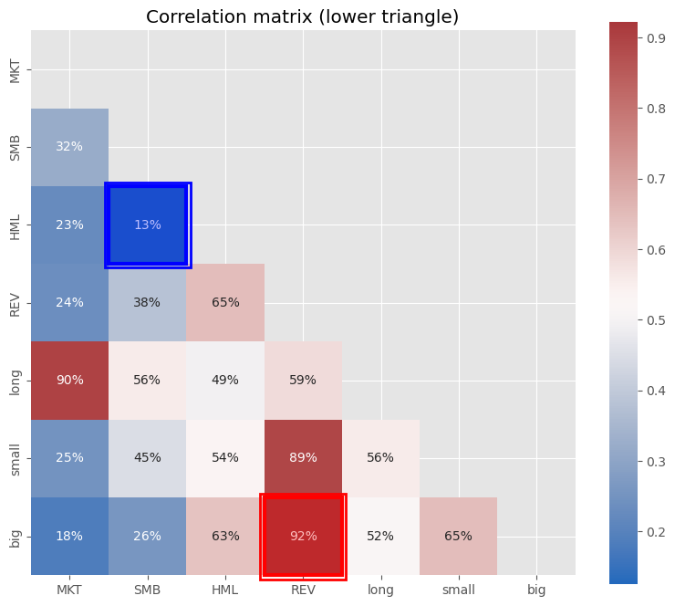
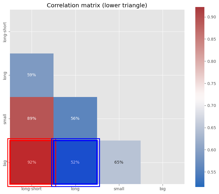
from cmds.plot_tools import plot_corr_matrix
temp = pd.concat([ff_factors[KEY], mom_long, mom_small, mom_large], axis=1)
temp.columns = ['long-short','long','small','big']

display(plot_corr_matrix(ff_factors,triangle='lower'));
display(plot_corr_matrix(temp,triangle='lower'));

(<Figure size 800x800 with 2 Axes>,
 <Axes: title={'center': 'Correlation matrix (lower triangle)'}>)

(<Figure size 800x800 with 2 Axes>,
 <Axes: title={'center': 'Correlation matrix (lower triangle)'}>)

display(plot_corr_matrix(pd.concat([ff_factors,temp.iloc[:,1:]],axis=1),triangle='lower'));

(<Figure size 800x800 with 2 Axes>,
 <Axes: title={'center': 'Correlation matrix (lower triangle)'}>)