Exercise - Unconstrained Optimization

Data

All the analysis below applies to the data set,

• data/spx_weekly_returns.xlsx

• The file has weekly returns.

• For annualization, use 52 periods per year.

Consider only the following 10 stocks…

TICKS =  ['AAPL','NVDA','MSFT','GOOGL','AMZN','META','TSLA','AVGO','BRK/B','LLY']

As well as the ETF,

TICK_ETF = 'SPY'

Data Processing

import pandas as pd

INFILE = '../data/spx_returns_weekly.xlsx'
SHEET_INFO = 's&p500 names'
SHEET_RETURNS = 's&p500 rets'
SHEET_BENCH = 'benchmark rets'

FREQ = 52

info = pd.read_excel(INFILE,sheet_name=SHEET_INFO)
info.set_index('ticker',inplace=True)
temp_mkt_cap = info.loc[TICKS].copy()
temp_mkt_cap['mkt cap'] /= 1e9
temp_mkt_cap.rename(columns={'mkt cap':'mkt cap (billions $)'},inplace=True)
temp_mkt_cap.style.format({'mkt cap (billions $)':'{:,.0f}'})

	name	mkt cap (billions $)
ticker
AAPL	Apple Inc	3,009
NVDA	NVIDIA Corp	3,480
MSFT	Microsoft Corp	3,514
GOOGL	Alphabet Inc	2,146
AMZN	Amazon.com Inc	2,304
META	Meta Platforms Inc	1,745
TSLA	Tesla Inc	994
AVGO	Broadcom Inc	1,149
BRK/B	Berkshire Hathaway Inc	1,064
LLY	Eli Lilly & Co	733

rets = pd.read_excel(INFILE,sheet_name=SHEET_RETURNS)
rets.set_index('date',inplace=True)
rets = rets[TICKS]

bench = pd.read_excel(INFILE,sheet_name=SHEET_BENCH)
bench.set_index('date',inplace=True)
rets[TICK_ETF] = bench[TICK_ETF]

---

1. Risk Statistics

1.1.

Display a table with the following metrics for each of the return series.

• mean (annualized)

• volatility (annualized)

• Sharpe ratio (annualized)

• skewness

• kurtosis

• maximum drawdown

Note

We have total returns, and Sharpe ratio is technically defined for excess returns. Don’t worry about the difference. (Or subtract SHV if you prefer.)

1.2.

As a standalone investment, which is most attractive? And least? Justify your answer.

1.3.

For each investment, estimate a regression against SPY. Report the

• alpha (annualized as a mean)

• beta

• info ratio

• r-squared

Based on this table, which investment seems most attractive relative to holding SPY?

---

import numpy as np
pd.options.display.float_format = "{:,.4f}".format

import matplotlib.pyplot as plt
import seaborn as sns

import statsmodels.api as sm
from sklearn.linear_model import LinearRegression

%matplotlib inline
plt.rcParams['figure.figsize'] = (12,6)
plt.rcParams['font.size'] = 15
plt.rcParams['legend.fontsize'] = 13

from cmds.portfolio import performanceMetrics, maximumDrawdown, get_ols_metrics
from cmds.risk import *

Solution 1.1.

mets = performanceMetrics(rets,annualization=FREQ)
mets['skewness'] = rets.skew()
mets['kurtosis'] = rets.kurtosis()
mets['max drawdown'] = maximumDrawdown(rets)['Max Drawdown']
mets.style.format('{:.1%}')

	Mean	Vol	Sharpe	Min	Max	skewness	kurtosis	max drawdown
AAPL	23.9%	27.7%	86.3%	-17.5%	14.7%	-21.9%	182.6%	-34.6%
NVDA	64.6%	46.3%	139.3%	-20.1%	30.2%	34.5%	138.9%	-65.9%
MSFT	26.1%	24.0%	108.9%	-14.4%	15.0%	7.2%	234.2%	-35.1%
GOOGL	21.7%	28.0%	77.5%	-12.0%	25.8%	58.3%	372.1%	-41.9%
AMZN	29.3%	30.6%	95.9%	-14.5%	18.5%	6.3%	178.2%	-54.8%
META	26.2%	35.1%	74.6%	-23.7%	24.5%	5.2%	402.4%	-76.0%
TSLA	47.0%	58.6%	80.1%	-25.9%	33.3%	54.8%	159.4%	-72.2%
AVGO	39.5%	37.5%	105.3%	-18.3%	25.2%	66.2%	350.4%	-40.0%
BRK/B	13.5%	19.1%	70.8%	-13.4%	9.8%	-20.1%	251.3%	-26.5%
LLY	28.2%	28.3%	99.5%	-12.2%	17.5%	21.6%	168.3%	-25.3%
SPY	13.1%	17.1%	76.8%	-14.5%	12.1%	-57.9%	599.6%	-31.8%

Solution 1.2.

As a standalone investment, NVDA has

• the best Sharpe, which is the best vol-adjusted return.

• large positive skewness which is attractive.

• large kurtosis, which would be bad with negative skewness but is appealing with positive skewness.

• a large max drawdown.

If worried about the max drawdown, LLY may be a good choice.

• smallest max drawdown

• still has 4th hgihest Sharpe.

Solution 1.3.

get_ols_metrics(rets['SPY'],rets,FREQ).style.format('{:.1%}',na_rep='-')

	alpha	SPY	r-squared	Treynor Ratio	Info Ratio
AAPL	9.3%	111.3%	47.3%	21.4%	46.1%
NVDA	41.8%	173.5%	41.0%	37.2%	117.4%
MSFT	12.6%	103.2%	54.0%	25.3%	77.4%
GOOGL	7.7%	106.6%	42.4%	20.3%	36.2%
AMZN	15.3%	106.6%	35.5%	27.5%	62.4%
META	11.1%	114.8%	31.2%	22.8%	38.2%
TSLA	23.8%	176.2%	26.4%	26.7%	47.4%
AVGO	21.7%	135.7%	38.2%	29.1%	73.5%
BRK/B	2.8%	81.7%	53.6%	16.5%	21.4%
LLY	19.9%	62.7%	14.3%	44.9%	76.1%
SPY	0.0%	100.0%	100.0%	13.1%	-

Based on this table, NVDA is the most attractive. It not only has (by far) the highest alpha, but also the highest Info Ratio (which is the risk-adjusted alpha.)

Solution .

get_ols_metrics(rets[['SPY','NVDA']],rets[['AAPL']],FREQ).style.format('{:.1%}',na_rep='-')

	alpha	SPY	NVDA	r-squared	Info Ratio
AAPL	7.1%	102.2%	5.3%	47.7%	35.3%

For every $100 in AAPL, we would short 97.9 dollars of SPY and short 7.4 dollars of NVDA.

Solution 1.5.

The r-squared indicates how highly correlated our replication is to the target.

---

2. Portfolio Allocation

2.1.

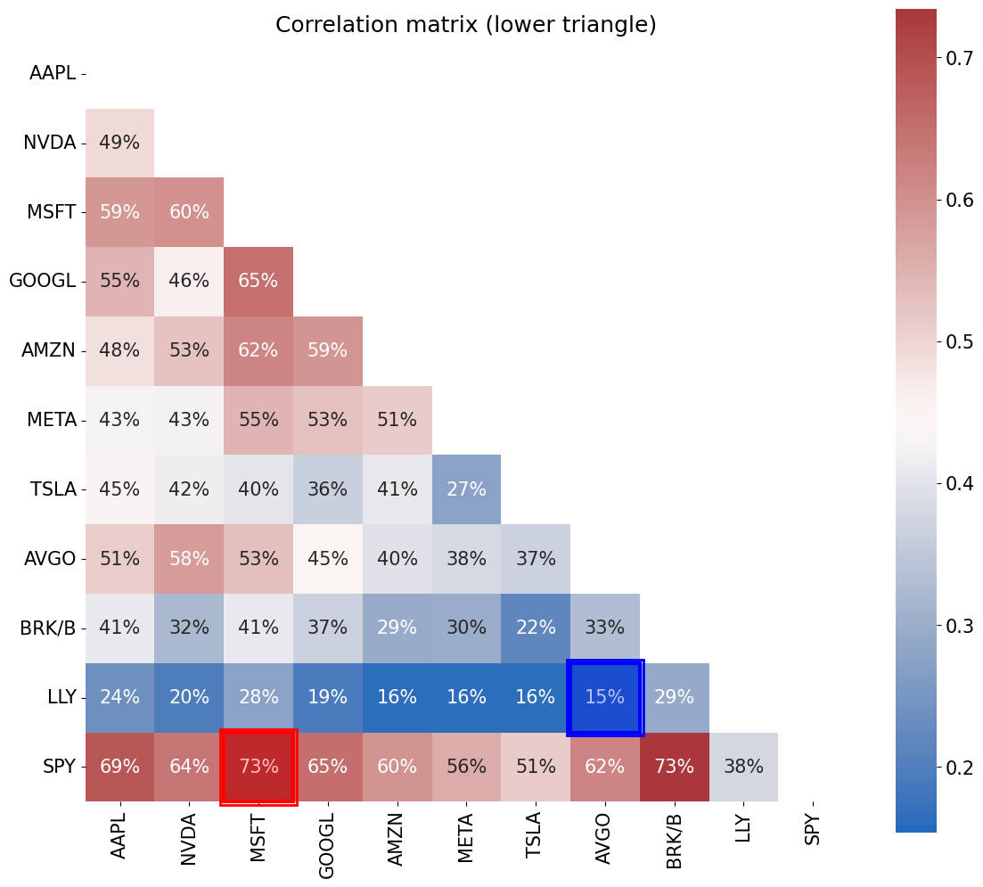
Display the correlation matrix of the returns.

• Based on this information, which investment do you anticipate will get extra weight in the portfolio, beyond what it would merit for its mean return?

• Report the maximally correlated assets and the minimally correlated assets.

2.2.

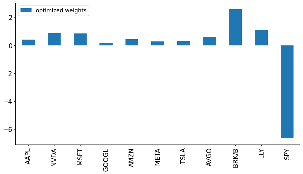
Calculate the weights of the mean-variance optimized portfolio, also called the tangency portfolio.

• Display a table indexed by each investment, with the optimal weights in one column and the Sharpe ratios in another column.

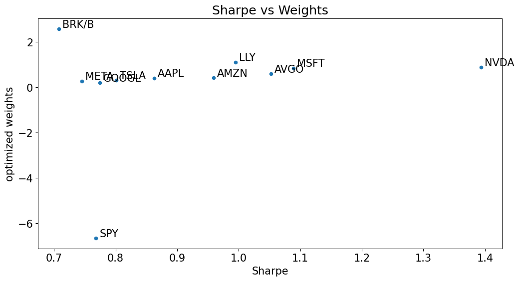
• Do the investments with the best Sharpe ratios tend to get the biggest weights?

Note:

To estimate the optimal weights, consider using the provided function below.

def optimized_weights(returns,dropna=True,scale_cov=1):
    if dropna:
        returns = returns.dropna()

    covmat_full = returns.cov()
    covmat_diag = np.diag(np.diag(covmat_full))
    covmat = scale_cov * covmat_full + (1-scale_cov) * covmat_diag

    weights = np.linalg.solve(covmat,returns.mean())
    weights = weights / weights.sum()

    if returns.mean() @ weights < 0:
        weights = -weights

    return pd.DataFrame(weights, index=returns.columns)

2.3.

Report the following performance statistics of the portfolio achieved with the optimized weights calculated above.

• mean

• volatility

• Sharpe

(Annualize all three statistics.)

2.4.

Try dropping the asset which had the biggest short position from the investment set. Re-run the optimization. What do you think of these new weights compared to the original optimized weights?

What is going on?

---

Solution 2.1

from cmds.plot_tools import plot_corr_matrix
plot_corr_matrix(rets,triangle='lower',figsize=(12,12))

(<Figure size 1200x1200 with 2 Axes>,
 <Axes: title={'center': 'Correlation matrix (lower triangle)'}>)

Solution 2.2

wts = pd.DataFrame(index=rets.columns)
wts['optimized weights'] = optimized_weights(rets)

wts.plot.bar();

sharpe_vs_wts = pd.concat([wts['optimized weights'],mets['Sharpe']],axis=1)
sharpe_vs_wts.sort_values('optimized weights',ascending=False).style.format('{:.1%}')

	optimized weights	Sharpe
BRK/B	258.0%	70.8%
LLY	111.3%	99.5%
NVDA	88.3%	139.3%
MSFT	84.9%	108.9%
AVGO	60.2%	105.3%
AMZN	42.6%	95.9%
AAPL	40.9%	86.3%
TSLA	31.0%	80.1%
META	27.7%	74.6%
GOOGL	19.3%	77.5%
SPY	-664.3%	76.8%

sharpe_vs_wts.plot.scatter(x='Sharpe',y='optimized weights')


for idx in sharpe_vs_wts.index:
    x_value = sharpe_vs_wts.loc[idx, "Sharpe"]
    y_value = sharpe_vs_wts.loc[idx, "optimized weights"]
    
    plt.annotate(
        text=idx,               
        xy=(x_value, y_value),  
        xytext=(5, 2),          
        textcoords="offset points"
    )

plt.xlabel("Sharpe")
plt.ylabel("optimized weights")
plt.title("Sharpe vs Weights")
plt.show()

Solution 2.3

port = pd.DataFrame(rets @ wts['optimized weights'],columns=['optimized weights'])
performanceMetrics(port,annualization=FREQ).style.format('{:.2%}')

	Mean	Vol	Sharpe	Min	Max
optimized weights	130.22%	62.95%	206.85%	-27.41%	32.35%

Solution 2.4

The optimization is unrealistic in that it prescribes massive positions.

• SPY is short nearly 600%.

• BRK-B is long nearly 200%.

Solution 2.5

The optimizer is shorting SPY because…

• it has lower mean return than the tech stocks (NVDA)

• it is highly correlated to the tech stocks and can offset much of their risk.

The optimizer is massively long BRK…

• even though BRK has the worst Sharpe ratio of the investments.

• But BRK is highly correlated to SPY while having relatively low correlation to tech. Thus it lowers total risk.

---

Extra: Sensitivity to dropping SPY

DROPTICK = 'SPY'

wts[f'optimized ex {DROPTICK}'] = optimized_weights(rets.drop(columns=[DROPTICK]))
wts.loc[f'{DROPTICK}',f'optimized ex {DROPTICK}'] = 0

port[f'optimized ex {DROPTICK}'] = pd.DataFrame(rets @ wts[f'optimized ex {DROPTICK}'],columns=[f'optimized ex {DROPTICK}'])

wts[f'optimized ex {DROPTICK}'].plot.bar();
plt.title(f'Weights - dropped {DROPTICK}');

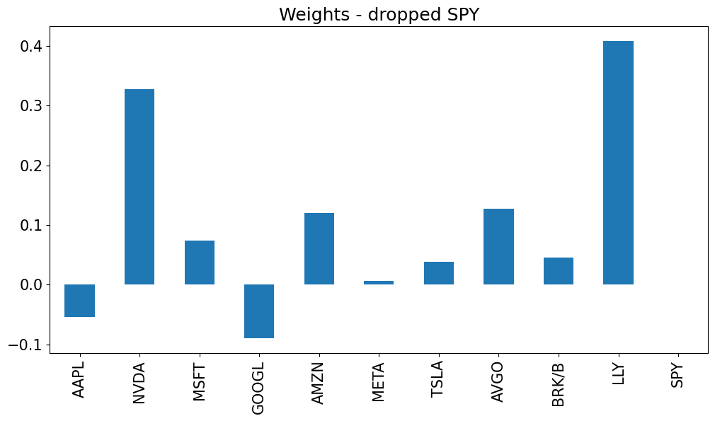
These weights are much more realistic. They are reasonable magnitudes and don’t include massive short positions.

Without SPY, the correlation matrix has relatively low correlations. Thus, the optimizer doesn’t think it can achieve such balanced (hedged) offsets, so it doesn’t prescribe extremes.

performanceMetrics(port,annualization=FREQ).style.format('{:.1%}')

	Mean	Vol	Sharpe	Min	Max
optimized weights	130.2%	63.0%	206.9%	-27.4%	32.3%
optimized ex SPY	42.4%	26.2%	161.6%	-11.9%	15.2%

wts.abs().sum().to_frame('gross mkt weight').style.format('{:,.1%}')

	gross mkt weight
optimized weights	1,428.6%
optimized ex SPY	128.9%