Statistics of the DFA Factors#
import numpy as np
import pandas as pd
pd.options.display.float_format = "{:,.4f}".format

import matplotlib.pyplot as plt
import seaborn as sns

import statsmodels.api as sm
from sklearn.linear_model import LinearRegression

from scipy import stats
import matplotlib.pyplot as plt
%matplotlib inline
plt.rcParams['figure.figsize'] = (12,6)
plt.rcParams['font.size'] = 15
plt.rcParams['legend.fontsize'] = 13
This uses factor_pricing.py, which you do not have.#
Thus, this notebook is just for demonstration.#
import sys
sys.path.insert(0, '../cmds')
sys.path.insert(0, '../DEV')
from portfolio import *
from factor_pricing import *
Load Data#
filepath_data = '../data/dfa_analysis_data.xlsx'
info = pd.read_excel(filepath_data,sheet_name='descriptions')
info.rename(columns={'Unnamed: 0':'Symbol'},inplace=True)
info.set_index('Symbol',inplace=True)

facs = pd.read_excel(filepath_data,sheet_name='factors')
facs.set_index('Date',inplace=True)
rf = facs['RF'].copy()
facs.drop(columns=['RF'],inplace=True)
2. Factors#
2.1#
dts = dict()
dts['early'] = pd.date_range(start=facs.index[0], end='31/12/1980',freq='M')
dts['founding'] = pd.date_range(start='1/1/1981', end='31/12/2001',freq='M')
dts['recent'] = pd.date_range(start='1/1/2002', end=facs.index[-1],freq='M')

dts['1990s'] = pd.date_range(start='1/1/1991', end='31/12/1999',freq='M')
dts['modern'] = dts['founding'].union(dts['recent'])
dts['all'] = facs.index
/var/folders/zx/3v_qt0957xzg3nqtnkv007d00000gn/T/ipykernel_92294/4220933265.py:2: FutureWarning: 'M' is deprecated and will be removed in a future version, please use 'ME' instead.
  dts['early'] = pd.date_range(start=facs.index[0], end='31/12/1980',freq='M')
/var/folders/zx/3v_qt0957xzg3nqtnkv007d00000gn/T/ipykernel_92294/4220933265.py:3: FutureWarning: 'M' is deprecated and will be removed in a future version, please use 'ME' instead.
  dts['founding'] = pd.date_range(start='1/1/1981', end='31/12/2001',freq='M')
/var/folders/zx/3v_qt0957xzg3nqtnkv007d00000gn/T/ipykernel_92294/4220933265.py:4: FutureWarning: 'M' is deprecated and will be removed in a future version, please use 'ME' instead.
  dts['recent'] = pd.date_range(start='1/1/2002', end=facs.index[-1],freq='M')
/var/folders/zx/3v_qt0957xzg3nqtnkv007d00000gn/T/ipykernel_92294/4220933265.py:6: FutureWarning: 'M' is deprecated and will be removed in a future version, please use 'ME' instead.
  dts['1990s'] = pd.date_range(start='1/1/1991', end='31/12/1999',freq='M')
for era in dts.keys():
    print(f'\n========================================================\n')
    print(f'Period: {dts[era][0]} to {dts[era][-1]}')
    print(f'\n========================================================')
    display(performanceMetrics(facs.loc[dts[era]],annualization=12).join(tailMetrics(facs.loc[dts[era]],quantile=.05)['VaR (0.05)']))
========================================================

Period: 1926-07-31 00:00:00 to 1980-12-31 00:00:00

========================================================
| Mean | Vol | Sharpe | Min | Max | VaR (0.05) | |
|---|---|---|---|---|---|---|
| Mkt-RF | 0.0810 | 0.2050 | 0.3949 | -0.2874 | 0.3881 | -0.0841 |
| SMB | 0.0339 | 0.1143 | 0.2968 | -0.0989 | 0.3596 | -0.0419 |
| HML | 0.0503 | 0.1342 | 0.3749 | -0.1319 | 0.3552 | -0.0442 |
========================================================

Period: 1981-01-31 00:00:00 to 2001-12-31 00:00:00

========================================================
| Mean | Vol | Sharpe | Min | Max | VaR (0.05) | |
|---|---|---|---|---|---|---|
| Mkt-RF | 0.0779 | 0.1572 | 0.4953 | -0.2319 | 0.1245 | -0.0641 |
| SMB | -0.0020 | 0.1173 | -0.0172 | -0.1741 | 0.2125 | -0.0459 |
| HML | 0.0646 | 0.1099 | 0.5876 | -0.0977 | 0.1224 | -0.0416 |
========================================================

Period: 2002-01-31 00:00:00 to 2025-08-31 00:00:00

========================================================
| Mean | Vol | Sharpe | Min | Max | VaR (0.05) | |
|---|---|---|---|---|---|---|
| Mkt-RF | 0.0913 | 0.1535 | 0.5947 | -0.1720 | 0.1360 | -0.0773 |
| SMB | 0.0079 | 0.0884 | 0.0897 | -0.0593 | 0.0714 | -0.0392 |
| HML | 0.0012 | 0.1064 | 0.0113 | -0.1383 | 0.1286 | -0.0415 |
========================================================

Period: 1991-01-31 00:00:00 to 1999-12-31 00:00:00

========================================================
| Mean | Vol | Sharpe | Min | Max | VaR (0.05) | |
|---|---|---|---|---|---|---|
| Mkt-RF | 0.1556 | 0.1298 | 1.1988 | -0.1605 | 0.1085 | -0.0416 |
| SMB | -0.0007 | 0.1042 | -0.0070 | -0.0694 | 0.0848 | -0.0501 |
| HML | 0.0142 | 0.0922 | 0.1539 | -0.0766 | 0.0651 | -0.0406 |
========================================================

Period: 1981-01-31 00:00:00 to 2025-08-31 00:00:00

========================================================
| Mean | Vol | Sharpe | Min | Max | VaR (0.05) | |
|---|---|---|---|---|---|---|
| Mkt-RF | 0.0850 | 0.1551 | 0.5478 | -0.2319 | 0.1360 | -0.0723 |
| SMB | 0.0033 | 0.1029 | 0.0316 | -0.1741 | 0.2125 | -0.0418 |
| HML | 0.0310 | 0.1083 | 0.2860 | -0.1383 | 0.1286 | -0.0415 |
========================================================

Period: 1926-07-31 00:00:00 to 2025-08-31 00:00:00

========================================================
| Mean | Vol | Sharpe | Min | Max | VaR (0.05) | |
|---|---|---|---|---|---|---|
| Mkt-RF | 0.0828 | 0.1841 | 0.4495 | -0.2874 | 0.3881 | -0.0792 |
| SMB | 0.0201 | 0.1093 | 0.1839 | -0.1741 | 0.3596 | -0.0418 |
| HML | 0.0416 | 0.1232 | 0.3377 | -0.1383 | 0.3552 | -0.0424 |
2.2#
Regarding the factor premia, we see that…
SMB premium is small in most subsamples and is negative during 1981-2001.
HML is positive overall and in most subsamples, but it is negative in the post-case sample of 2002-2021.
HML’s premium drops substantially starting in the 1990’s.
MKT is positive in every subsample, and strongly so.
2.3#
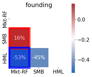
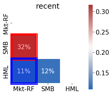
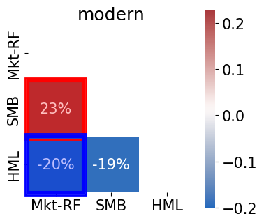
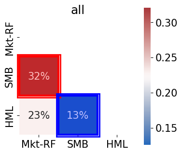
The correlations are low relative to most equity portfolios (which tend to have high correlations.)
The correlation between MKT and SMB is relatively low, but definitely positive.
The correlation between MKT and HML is negative since DFA’s founding, but it was positive before that, such that the 100-year sample is positive.
from cmds.plot_tools import plot_corr_matrix

for era in ['founding','recent','modern','all']:
    plot_corr_matrix(facs.loc[dts[era]],figsize=(4,4),triangle='lower');
    plt.title(era);
    plt.show()
(<Figure size 400x400 with 2 Axes>,
 <Axes: title={'center': 'Correlation matrix (lower triangle)'}>)
Text(0.5, 1.0, 'founding')
(<Figure size 400x400 with 2 Axes>,
 <Axes: title={'center': 'Correlation matrix (lower triangle)'}>)
Text(0.5, 1.0, 'recent')
(<Figure size 400x400 with 2 Axes>,
 <Axes: title={'center': 'Correlation matrix (lower triangle)'}>)
Text(0.5, 1.0, 'modern')
(<Figure size 400x400 with 2 Axes>,
 <Axes: title={'center': 'Correlation matrix (lower triangle)'}>)
Text(0.5, 1.0, 'all')
2.4#
display((1+facs.loc[dts['founding']]).cumprod().plot());
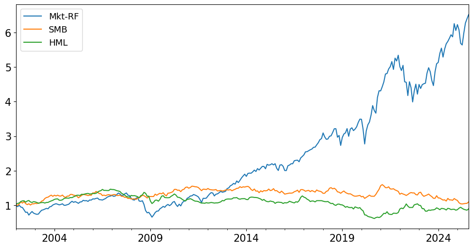
display((1+facs.loc[dts['recent']]).cumprod().plot());
<Axes: >
<Axes: >
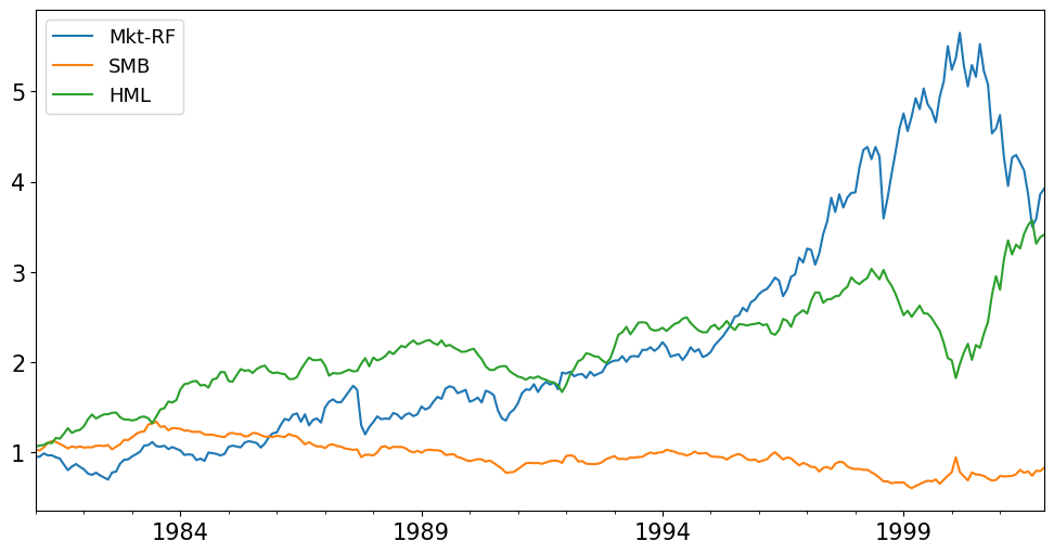
The plots above show that HML had high returns in the era of the case: 1981-2001.
In the post-case period (2002-2021) HML has a negative mean return. Nonetheless, it may be valuable given that it has negative correlation to MKT during this time.
However, SMB has small or negative returns in this period while being positively correlated to MKT. Thus, it may be reasonable to drop SMB.
Tangency Weights of Factors#
Another way to consider whether all three factors matter is to remember that if a factor prices, then by the Fundamental Theorem of Asset Pricing it must be part of the tangency portfolio.
Calculate the tangency portfolio formed by the factors. Do they all get substantial weight? We see that SMB has very little weight in the three-factor Tangency portfolio.
Thus, we again see that SMB may be unnecessary.
3. CAPM#
3.1#
# load data
rets = pd.read_excel(filepath_data,sheet_name='portfolios (total returns)')
rets.set_index('Date',inplace=True)
# excess portfolio returns
retsx = rets.subtract(rf,axis=0)
# subsample of modern
facsT = facs.loc[dts['modern']]
retsxT = retsx.loc[dts['modern']]
mets = performanceMetrics(retsxT,annualization=12)
tail = tailMetrics(retsxT)

display(mets.join(tail['VaR (0.05)']))
| Mean | Vol | Sharpe | Min | Max | VaR (0.05) | |
|---|---|---|---|---|---|---|
| SMALL LoBM | 0.0117 | 0.2717 | 0.0431 | -0.3477 | 0.3596 | -0.1249 |
| ME1 BM2 | 0.0884 | 0.2354 | 0.3756 | -0.3128 | 0.4309 | -0.0949 |
| ME1 BM3 | 0.0902 | 0.2008 | 0.4493 | -0.2919 | 0.1999 | -0.0848 |
| ME1 BM4 | 0.1125 | 0.1940 | 0.5800 | -0.2896 | 0.2563 | -0.0776 |
| SMALL HiBM | 0.1273 | 0.2084 | 0.6110 | -0.2908 | 0.4121 | -0.0882 |
| ME2 BM1 | 0.0609 | 0.2447 | 0.2490 | -0.3308 | 0.3024 | -0.1032 |
| ME2 BM2 | 0.0984 | 0.2054 | 0.4790 | -0.3254 | 0.1892 | -0.0834 |
| ME2 BM3 | 0.1052 | 0.1864 | 0.5640 | -0.2926 | 0.1832 | -0.0803 |
| ME2 BM4 | 0.1081 | 0.1819 | 0.5942 | -0.2526 | 0.1869 | -0.0753 |
| ME2 BM5 | 0.1132 | 0.2137 | 0.5298 | -0.3209 | 0.2596 | -0.0933 |
| ME3 BM1 | 0.0694 | 0.2237 | 0.3103 | -0.3030 | 0.2217 | -0.0995 |
| ME3 BM2 | 0.1040 | 0.1871 | 0.5555 | -0.2908 | 0.1874 | -0.0786 |
| ME3 BM3 | 0.0910 | 0.1729 | 0.5264 | -0.2551 | 0.1669 | -0.0732 |
| ME3 BM4 | 0.1053 | 0.1797 | 0.5863 | -0.2667 | 0.1666 | -0.0722 |
| ME3 BM5 | 0.1240 | 0.2024 | 0.6125 | -0.3131 | 0.2291 | -0.0845 |
| ME4 BM1 | 0.0919 | 0.2008 | 0.4575 | -0.2615 | 0.2538 | -0.0835 |
| ME4 BM2 | 0.0937 | 0.1761 | 0.5323 | -0.2929 | 0.1553 | -0.0723 |
| ME4 BM3 | 0.0920 | 0.1742 | 0.5282 | -0.2514 | 0.1681 | -0.0762 |
| ME4 BM4 | 0.1059 | 0.1741 | 0.6081 | -0.3220 | 0.1627 | -0.0688 |
| ME4 BM5 | 0.1056 | 0.1990 | 0.5307 | -0.3264 | 0.2037 | -0.0857 |
| BIG LoBM | 0.0949 | 0.1634 | 0.5807 | -0.2225 | 0.1490 | -0.0758 |
| ME5 BM2 | 0.0857 | 0.1544 | 0.5552 | -0.2305 | 0.1607 | -0.0641 |
| ME5 BM3 | 0.0796 | 0.1529 | 0.5211 | -0.2263 | 0.1425 | -0.0711 |
| ME5 BM4 | 0.0726 | 0.1704 | 0.4258 | -0.2759 | 0.1636 | -0.0738 |
| BIG HiBM | 0.1035 | 0.2040 | 0.5076 | -0.2858 | 0.2199 | -0.0890 |
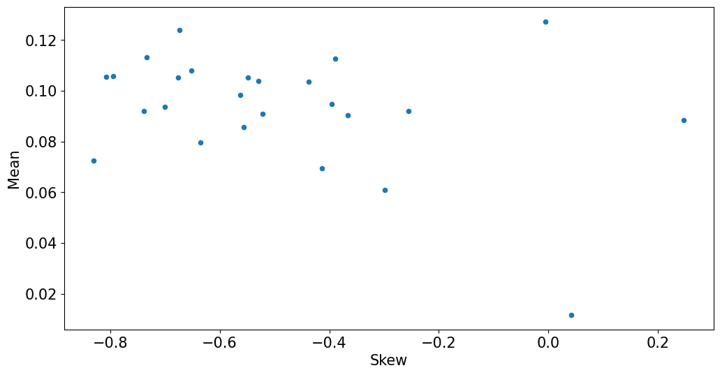
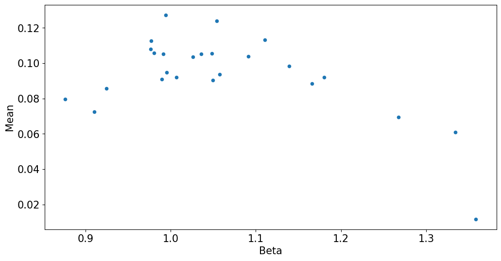
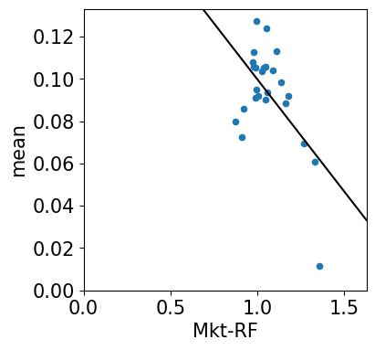
Explaining premia by risk metrics#
lfd = get_ols_metrics(facsT['Mkt-RF'],retsxT,annualization=12)
mets['Beta'] = lfd[['Mkt-RF']]
mets['VaR'] = tail[['VaR (0.05)']]
mets['Skew'] = tail[['Skewness']]
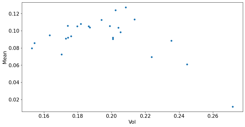
mets.plot.scatter(x='Vol',y='Mean');
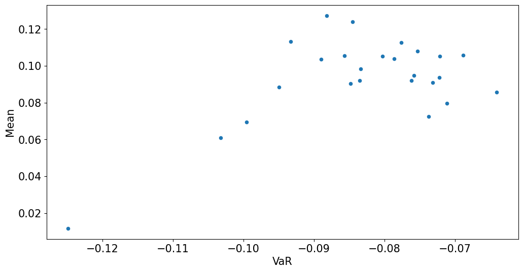
mets.plot.scatter(x='VaR',y='Mean');
mets.plot.scatter(x='Skew',y='Mean');
mets.plot.scatter(x='Beta',y='Mean');
3.2 CAPM Tests: Time-Series Metrics#
display(lfd)
| alpha | Mkt-RF | r-squared | Treynor Ratio | Info Ratio | |
|---|---|---|---|---|---|
| SMALL LoBM | -0.1037 | 1.3585 | 0.6014 | 0.0086 | -0.6047 |
| ME1 BM2 | -0.0106 | 1.1658 | 0.5900 | 0.0759 | -0.0705 |
| ME1 BM3 | 0.0010 | 1.0495 | 0.6571 | 0.0860 | 0.0088 |
| ME1 BM4 | 0.0295 | 0.9773 | 0.6105 | 0.1151 | 0.2435 |
| SMALL HiBM | 0.0429 | 0.9939 | 0.5476 | 0.1281 | 0.3058 |
| ME2 BM1 | -0.0524 | 1.3341 | 0.7154 | 0.0457 | -0.4018 |
| ME2 BM2 | 0.0016 | 1.1390 | 0.7401 | 0.0864 | 0.0151 |
| ME2 BM3 | 0.0171 | 1.0357 | 0.7426 | 0.1015 | 0.1812 |
| ME2 BM4 | 0.0251 | 0.9765 | 0.6937 | 0.1107 | 0.2493 |
| ME2 BM5 | 0.0188 | 1.1108 | 0.6505 | 0.1019 | 0.1488 |
| ME3 BM1 | -0.0383 | 1.2677 | 0.7725 | 0.0548 | -0.3589 |
| ME3 BM2 | 0.0112 | 1.0911 | 0.8179 | 0.0953 | 0.1408 |
| ME3 BM3 | 0.0069 | 0.9895 | 0.7879 | 0.0920 | 0.0872 |
| ME3 BM4 | 0.0211 | 0.9911 | 0.7320 | 0.1063 | 0.2271 |
| ME3 BM5 | 0.0344 | 1.0543 | 0.6528 | 0.1176 | 0.2883 |
| ME4 BM1 | -0.0084 | 1.1800 | 0.8308 | 0.0779 | -0.1016 |
| ME4 BM2 | 0.0038 | 1.0577 | 0.8685 | 0.0886 | 0.0600 |
| ME4 BM3 | 0.0065 | 1.0068 | 0.8036 | 0.0914 | 0.0838 |
| ME4 BM4 | 0.0226 | 0.9803 | 0.7630 | 0.1080 | 0.2662 |
| ME4 BM5 | 0.0165 | 1.0484 | 0.6679 | 0.1007 | 0.1439 |
| BIG LoBM | 0.0103 | 0.9955 | 0.8935 | 0.0953 | 0.1926 |
| ME5 BM2 | 0.0071 | 0.9247 | 0.8631 | 0.0927 | 0.1249 |
| ME5 BM3 | 0.0052 | 0.8760 | 0.7904 | 0.0909 | 0.0743 |
| ME5 BM4 | -0.0048 | 0.9102 | 0.6863 | 0.0797 | -0.0501 |
| BIG HiBM | 0.0164 | 1.0260 | 0.6087 | 0.1009 | 0.1282 |
If CAPM were true, then we would have the following implications:
Treynor ratio would be the same for every asset, and it would equal the MKT premium.
The alphas would all be zero
The Information Ratios would all be zero
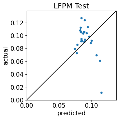
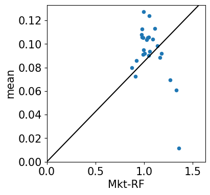
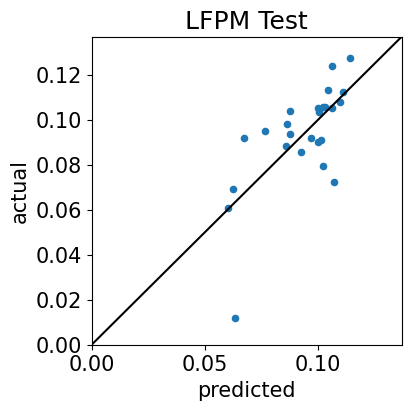
3.3 Cross-Sectional Test: Yes Intercept#
LFPtests(retsxT,facsT[['Mkt-RF']],annualization=12,useIntCS=True)
Time-Series Test Plots
Cross-Sectional Test Plots
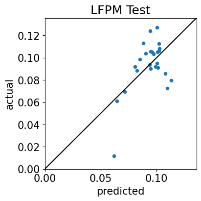
ESTIMATES
| premium-TS | premium-CS | |
|---|---|---|
| Mkt-RF | 0.0850 | -0.1059 |
| intercept | NaN | 0.2058 |
MODEL FIT
| MAE-TS | MAE-CS | rsquared | |
|---|---|---|---|
| error | 0.0207 | 0.0141 | 0.3132 |
STATISTICAL SIGNIFICANCE
| time-series | priced | premium |
|---|---|---|
| p-values | ||
| Mkt-RF | 0.0003 | 0.0001 |
| error | 0.0000 | NaN |
"premium" p-value is the usual t-stat on the time-series factor mean.
"priced" p-value of factor is the t-stat of forming the tangency portfolio.
"priced" p-value of "error" is the joint-chi-squared test of the time-series alphas
3.4#
These results support the idea that the MKT premium is not sufficient for explaining all premia in the market.
Given that MKT cannot explain these assets, which are sorted by size and value, it is suggestive that there may be premia in size and value.
But while we have ruled out MKT as being the only determinant factor, we have not proven size and value matter.
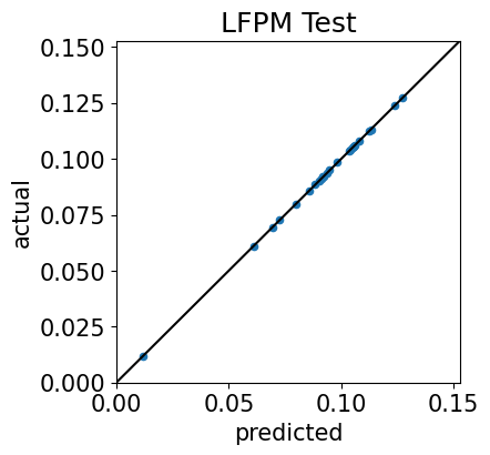
4.1 Fama-French 3-Factor Tests#
Time-Series Test#
Cross-Sectional Test: YES Intercept#
LFPtests(retsxT,facsT,annualization=12,useIntCS=True)
Time-Series Test Plots
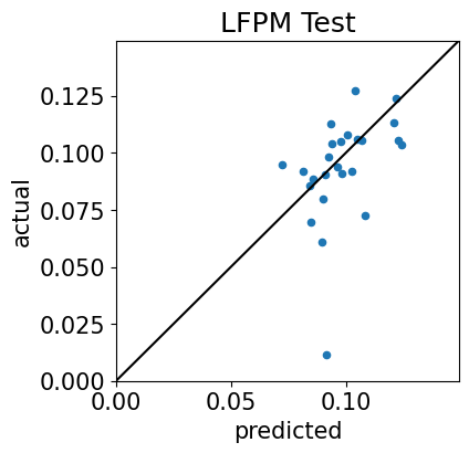
Cross-Sectional Test Plots
ESTIMATES
| premium-TS | premium-CS | |
|---|---|---|
| HML | 0.0310 | 0.0346 |
| Mkt-RF | 0.0850 | -0.0937 |
| SMB | 0.0033 | -0.0025 |
| intercept | NaN | 0.1800 |
MODEL FIT
| MAE-TS | MAE-CS | rsquared | |
|---|---|---|---|
| error | 0.0141 | 0.0114 | 0.4798 |
STATISTICAL SIGNIFICANCE
| time-series | priced | premium |
|---|---|---|
| p-values | ||
| Mkt-RF | 0.0001 | 0.0001 |
| SMB | 0.8189 | 0.4163 |
| HML | 0.0098 | 0.0282 |
| error | 0.0000 | NaN |
"premium" p-value is the usual t-stat on the time-series factor mean.
"priced" p-value of factor is the t-stat of forming the tangency portfolio.
"priced" p-value of "error" is the joint-chi-squared test of the time-series alphas
4.2 Tangency Tests#
Time-Series Test#
Cross-Sectional Test: Yes Intercept#
tangency = retsxT @ tangency_weights(retsxT)
tangency.columns= ['Tangency']

LFPtests(retsxT,tangency,annualization=12,useIntCS=True)
Time-Series Test Plots
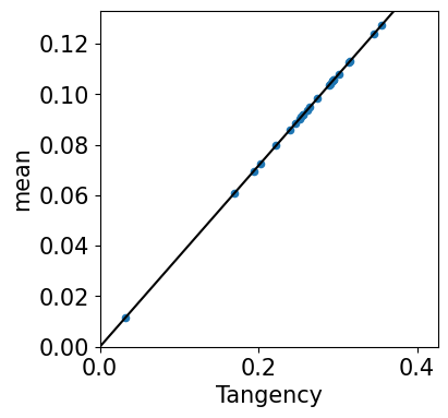
Cross-Sectional Test Plots
ESTIMATES
| premium-TS | premium-CS | |
|---|---|---|
| Tangency | 0.3584 | 0.3584 |
| intercept | NaN | 0.0000 |
MODEL FIT
| MAE-TS | MAE-CS | rsquared | |
|---|---|---|---|
| error | 0.0000 | 0.0000 | 1.0000 |
STATISTICAL SIGNIFICANCE
| time-series | priced | premium |
|---|---|---|
| p-values | ||
| Tangency | 0.0000 | 0.0000 |
| error | 1.0000 | NaN |
"premium" p-value is the usual t-stat on the time-series factor mean.
"priced" p-value of factor is the t-stat of forming the tangency portfolio.
"priced" p-value of "error" is the joint-chi-squared test of the time-series alphas
4.3#
The MAE#
is shown in the tables above labeled as MODEL FIT.
Joint Test of Alphas#
These test stats can be found in the tables above labeled as “STATISTICAL SIGNIFICANCE” in the “error”,”priced” cell of the table.
We note that the p-value for CAPM is 0 to many decimal places.
So is the p-value for Fama-French 3 Factor.
However, the p-value for the Tangency factor is 1, meaning that its errors are certainly not significant–because they are 0 to machine precision.
Stricter test#
Checking individual alphas for significance via a t-test may rule out a model.
But checking a group of alphas for joint significance via a chi-squared test is a higher hurdle for the model. Even if no individual alpha is significant, the group may be significant. We see this in that the joint test p-values for CAPM and FF are 0 to many decimals.
Testing the Tangency#
The test statistic can be viewed as the squared Sharpe Ratio of the tangency portfolio formed by alphas compared to the squared Sharpe Ratio of the model tangency portfolio (formed via the factors).