Solution - Constrained Optimization#
Data#
All the analysis below applies to the data set,
data/spx_weekly_returns.xlsxThe file has weekly returns.
For annualization, use 52 periods per year.
Consider only the following 10 stocks…
TICKS = ['AAPL','NVDA','MSFT','GOOGL','AMZN','META','TSLA','AVGO','BRK/B','LLY']
As well as the ETF,
TICK_ETF = 'SPY'
Data Processing#
import pandas as pd
INFILE = '../data/spx_returns_weekly.xlsx'
SHEET_INFO = 's&p500 names'
SHEET_RETURNS = 's&p500 rets'
SHEET_BENCH = 'benchmark rets'

FREQ = 52
info = pd.read_excel(INFILE,sheet_name=SHEET_INFO)
info.set_index('ticker',inplace=True)
info.loc[TICKS]
| name | mkt cap | |
|---|---|---|
| ticker | ||
| AAPL | Apple Inc | 3.008822e+12 |
| NVDA | NVIDIA Corp | 3.480172e+12 |
| MSFT | Microsoft Corp | 3.513735e+12 |
| GOOGL | Alphabet Inc | 2.145918e+12 |
| AMZN | Amazon.com Inc | 2.303536e+12 |
| META | Meta Platforms Inc | 1.745094e+12 |
| TSLA | Tesla Inc | 9.939227e+11 |
| AVGO | Broadcom Inc | 1.148592e+12 |
| BRK/B | Berkshire Hathaway Inc | 1.064240e+12 |
| LLY | Eli Lilly & Co | 7.332726e+11 |
rets = pd.read_excel(INFILE,sheet_name=SHEET_RETURNS)
rets.set_index('date',inplace=True)
rets = rets[TICKS]
bench = pd.read_excel(INFILE,sheet_name=SHEET_BENCH)
bench.set_index('date',inplace=True)
rets[TICK_ETF] = bench[TICK_ETF]
1 Constrained Optimization for Mean-Variance#
Continue working with the data above. Suppose we want to constrain the weights such that
there are no short positions beyond negative
20%, \(w_i\ge -.20\) for all \(i\)none of the positions may have weight over
35%, \(w_i \le .35\) for all \(i\).all the asset weights must sum to 1
Furthermore,
The targeted mean return is
20%per year.Be careful; the target is an annualized mean.
Consider using the code below as a starting point.
1.1.#
Report the weights of the constrained portfolio.
Report the mean, volatility, and Sharpe ratio of the resulting portfolio.
1.2.#
Compare these weights to the assets’ Sharpe ratios and means.
Do the most extreme positions also have the most extreme Sharpe ratios and means?
Why?
1.3.#
Compare the bounded portfolio weights to the unbounded portfolio weights (obtained from optimizing without the inequality constraints, keeping the equality constraints.)
Report the mean, volatility, and Sharpe ratio of both.
Code Help#
The minimize function will be how we optimize.
from scipy.optimize import minimize
Build the objective functions.
Before doing this, you will need to define
TARGET_MEANFREQcovmean
# def objective(w):
#     return (w.T @ cov @ w)

# def fun_constraint_capital(w):
#     return np.sum(w) - 1

# def fun_constraint_mean(w):
#     return (mean @ w) - TARGET_MEAN
Build the constraints
sum of weights add to one
weighted average of means is the target mean
# constraint_capital = {'type': 'eq', 'fun': fun_constraint_capital}
# constraint_mean = {'type': 'eq', 'fun': fun_constraint_mean}

# constraints = ([constraint_capital, constraint_mean])
Build the upper and lower bounds on each asset.
You will need to use the minimize function along with these contraints, bounds, and an initial guess.
Solutions#
import pandas as pd
import numpy as np
import datetime
import warnings

import matplotlib.pyplot as plt
%matplotlib inline
plt.rcParams['figure.figsize'] = (10,5)
plt.rcParams['font.size'] = 13
plt.rcParams['legend.fontsize'] = 13

from matplotlib.ticker import (MultipleLocator,
                               FormatStrFormatter,
                               AutoMinorLocator)
from cmds.portfolio import *
from cmds.risk import *
#from cmds.plot_tools import plot_triangular_matrix

from cmds.mvportfolio import MVweights
def optimized_weights(returns,dropna=True,scale_cov=1):
    if dropna:
        returns = returns.dropna()

    covmat_full = returns.cov()
    covmat_diag = np.diag(np.diag(covmat_full))
    covmat = scale_cov * covmat_full + (1-scale_cov) * covmat_diag

    weights = np.linalg.solve(covmat,returns.mean())
    weights = weights / weights.sum()

    if returns.mean() @ weights < 0:
        weights = -weights

    return pd.DataFrame(weights, index=returns.columns)
1. Optimized Portfolios#
DO_EXCESS = True
USE_RF_ZERO = True
if USE_RF_ZERO:
    rf = 0
else:
    rf = bench['SHV']

retsx = rets.sub(rf)

if DO_EXCESS:
    r = retsx
else:
    r = rets
temp = performanceMetrics(r,annualization=FREQ).drop(columns=['Min','Max'])
temp.sort_values('Sharpe',ascending=False).style.format('{:.2%}',na_rep='')
| Mean | Vol | Sharpe | |
|---|---|---|---|
| NVDA | 64.56% | 46.33% | 139.35% |
| MSFT | 26.14% | 24.00% | 108.93% |
| AVGO | 39.49% | 37.51% | 105.26% |
| LLY | 28.15% | 28.30% | 99.49% |
| AMZN | 29.34% | 30.60% | 95.90% |
| AAPL | 23.87% | 27.66% | 86.29% |
| TSLA | 46.98% | 58.64% | 80.10% |
| GOOGL | 21.68% | 27.99% | 77.47% |
| SPY | 13.13% | 17.09% | 76.82% |
| META | 26.19% | 35.13% | 74.55% |
| BRK/B | 13.50% | 19.07% | 70.82% |
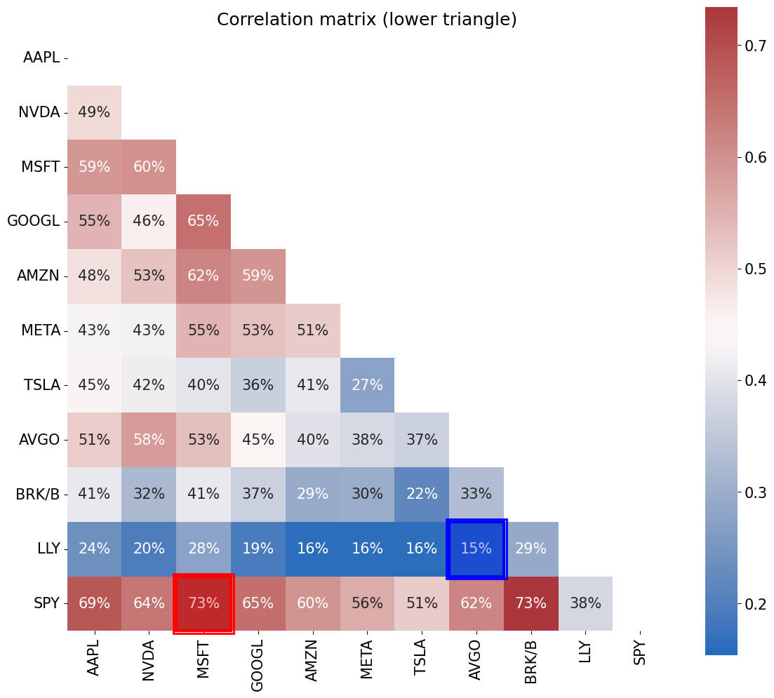
corr_matrix = r.corr()
from cmds.plot_tools import plot_corr_matrix
plot_corr_matrix(r,triangle='lower',figsize=(12,12))
plt.show()
mean = r.mean() * FREQ
cov = r.cov() * FREQ
Nassets = r.shape[1]
MINBOUND = -.10
MAXBOUND = .35
TARGET_MEAN = .20
def objective(w):
    return (w.T @ cov @ w)

def fun_constraint_capital(w):
    return np.sum(w) - 1

def fun_constraint_mean(w):
    return (mean @ w) - TARGET_MEAN

constraint_capital = {'type': 'eq', 'fun': fun_constraint_capital}
constraint_mean = {'type': 'eq', 'fun': fun_constraint_mean}

if DO_EXCESS:
    constraints = ([constraint_mean])
else:
    constraints = ([constraint_capital, constraint_mean])
bounds_df = pd.DataFrame(index=rets.columns,columns=['Min','Max'],dtype=float)
bounds_df['Min'] = MINBOUND
bounds_df['Max'] = MAXBOUND
bounds = [tuple(bounds_df.iloc[i,:].values) for i in range(Nassets)]
wstar = pd.DataFrame(index=temp.index,columns=['equal','bounded','unbounded'],dtype=float)
wstar['equal'] = np.ones(len(wstar.index))/Nassets
TOL = 1e-8
METHOD = 'SLSQP'
#METHOD = 'trust-constr'

w0 = np.ones(Nassets) / Nassets

solution_unbounded = minimize(objective, w0, method=METHOD, constraints=constraints, tol=TOL)
solution_bounded = minimize(objective, w0, method=METHOD, bounds=bounds, constraints=constraints, tol=TOL)
wstar['bounded'] = solution_bounded.x
wstar['unbounded'] = solution_unbounded.x

#wstar['analytic'] = optimized_weights(r,dropna=True,scale_cov=1)
wstar['analytic'] = MVweights(mean=mean,cov=cov,isexcess=DO_EXCESS,target=TARGET_MEAN)

if solution_bounded.success and solution_unbounded.success:
    print('Optimization SUCCESSFUL.')
else:
    print('Optimization FAILED.')

print(f'Iterations: {solution_bounded.nit}.')
Optimization SUCCESSFUL.
Iterations: 19.
1.1, 1.3. Portfolio Stats#
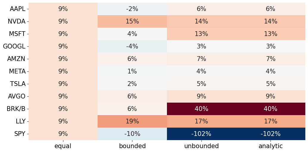
wstar.sort_values('bounded',ascending=False).style.format('{:.2%}')
| equal | bounded | unbounded | analytic | |
|---|---|---|---|---|
| LLY | 9.09% | 19.03% | 17.12% | 17.09% |
| NVDA | 9.09% | 15.30% | 13.55% | 13.56% |
| AVGO | 9.09% | 6.30% | 9.25% | 9.24% |
| AMZN | 9.09% | 5.80% | 6.52% | 6.55% |
| BRK/B | 9.09% | 5.75% | 39.63% | 39.63% |
| MSFT | 9.09% | 4.38% | 13.04% | 13.03% |
| TSLA | 9.09% | 2.07% | 4.76% | 4.76% |
| META | 9.09% | 0.66% | 4.27% | 4.26% |
| AAPL | 9.09% | -1.71% | 6.29% | 6.29% |
| GOOGL | 9.09% | -3.55% | 2.98% | 2.97% |
| SPY | 9.09% | -10.00% | -102.02% | -102.02% |
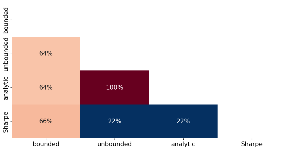
corr_weights = wstar.drop(columns=['equal']).corr().iloc[0,1]
display(f'Correlation between BOUNDED and UNBOUNDED is: {corr_weights:.1%}')
'Correlation between BOUNDED and UNBOUNDED is: 63.8%'
from cmds.plot_tools import plot_triangular_matrix
plot_triangular_matrix(wstar, full_matrix=True)
plt.show()
optimized = pd.DataFrame(index=['equal', 'bounded', 'unbounded'], columns=['mean','vol'],dtype=float)

optimized.loc['equal','mean'] = wstar['equal'] @ mean
optimized.loc['equal','vol'] = np.sqrt(wstar['equal'] @ cov @ wstar['equal'])

optimized.loc['bounded','mean'] = wstar['bounded'] @ mean
optimized.loc['bounded','vol'] = np.sqrt(wstar['bounded'] @ cov @ wstar['bounded'])

optimized.loc['unbounded','mean'] = wstar['unbounded'] @ mean
optimized.loc['unbounded','vol'] = np.sqrt(wstar['unbounded'] @ cov @ wstar['unbounded'])

optimized.loc['analytic','mean'] = wstar['analytic'] @ mean
optimized.loc['analytic','vol'] = np.sqrt(wstar['analytic'] @ cov @ wstar['analytic'])

optimized['sharpe'] = optimized['mean'] / optimized['vol']

optimized.style.format('{:.2%}')
| mean | vol | sharpe | |
|---|---|---|---|
| equal | 30.28% | 22.16% | 136.64% |
| bounded | 20.00% | 11.92% | 167.83% |
| unbounded | 20.00% | 9.67% | 206.85% |
| analytic | 20.00% | 9.67% | 206.85% |
1.2. Comparison with Stand-alone Metrics#
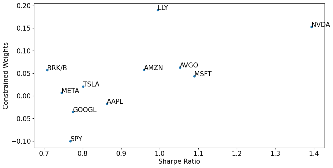
Consider how the most extreme positions compare to the most extreme Sharpe Ratios.
df = pd.concat([wstar[['bounded']],temp[['Sharpe']]],axis=1).sort_values('Sharpe',ascending=False)
ax = df.plot.scatter(x='Sharpe',y='bounded')
ax.set_xlabel('Sharpe Ratio')
ax.set_ylabel('Constrained Weights')
for idx, row in df.iterrows():
    ax.annotate(idx, (row['Sharpe'], row['bounded']))
temp = pd.concat([wstar,temp[['Sharpe']]],axis=1).drop(columns=['equal']).corr()
plot_triangular_matrix(temp,full_matrix=False)
Costs of the Bounds#
Using the LaGrangian…
warnings.filterwarnings("ignore", message="delta_grad == 0.0. Check if the approximated function is linear.")

TOL = 1e-12
METHOD = 'trust-constr'

w0 = wstar['bounded']
solutionALT = minimize(objective, w0, method=METHOD, bounds=bounds,constraints=constraints, tol=TOL)

pd.DataFrame(solutionALT.v[-1], index=mean.index, columns=['Lagrange Multipliers']).sort_values('Lagrange Multipliers',ascending=False).style.format('{:.2%}'.format)
| Lagrange Multipliers | |
|---|---|
| MSFT | 0.00% |
| AMZN | 0.00% |
| GOOGL | 0.00% |
| AAPL | 0.00% |
| AVGO | 0.00% |
| META | 0.00% |
| TSLA | 0.00% |
| BRK/B | -0.00% |
| NVDA | -0.00% |
| LLY | -0.00% |
| SPY | -1.05% |