Solution - Risk Metrics#
Data#
Try this exercise with data from
../data/risk_etf_data.xlsx../data/spx_returns_daily.xlsx
1. Risk Metrics of Stocks#
1.1 Return Moments#
Report the moments of the returns. Annualize the mean and volatility.
mean
volatility
skewness
(excess) kurtosis
Note that the pandas function for kurtosis already reports excess kurtosis.
1.2 Maximum Drawdown#
Report the maximum drawdown for each return series.
If we resampled this data to weekly and recalculated the maximum drawdown, do you think it would be larger or smaller (in magnitude)?
1.3 Quantiles#
Report the quantiles of the series. Use .describe() for a useful summary.
Report the 5th quantile scaled by standard deviation.
How much sampling error is in the mean return? Is this likely to cause much sampling error in the quantile estimation?
1.4 Comparison#
Try repeating 1.1-1.3 for another asset.
2. Time Aggregation#
Use the price series to calculate monthly returns. (You may find df.resample('M').last() helpful.
2.1 Measuring Covariation Risk#
When discussing asset correlation to SPY, does it matter whether we examine daily versus monthly returns?
Report the correlation between each asset and
SPYfor both daily and monthly returns.What do you conclude?
If using the “risk etf” data, consider the answer for BTC.
2.2 Betas#
For each series, calculate its beta to SPY.
Estimate the regression with an intercept (alpha) but no need to report it.
How do these betas compare to the daily return betas?
2.3 Time Scaling to Higher Moments#
Report the skewness and kurtosis for the monthly returns.
How do these compare to the daily skewness and kurtosis measures?
What do you conclude?
Solutions#
import pandas as pd
import numpy as np
import datetime

import matplotlib.pyplot as plt
%matplotlib inline
plt.rcParams['figure.figsize'] = (10,5)
plt.rcParams['font.size'] = 13
plt.rcParams['legend.fontsize'] = 13

from matplotlib.ticker import (MultipleLocator,
                               FormatStrFormatter,
                               AutoMinorLocator)

from cmds.portfolio import *
from cmds.risk import *
1#
Use SPX stock data#
# DATAPATH = f'../data/spx_returns_daily.xlsx'
# SHEET = 's&p500 rets'

# TICKS = [
#     'AAPL',
#     'META',
#     'NVDA',
#     'TSLA'
# ]

# FREQ = 252

# rets = pd.read_excel(DATAPATH, sheet_name=SHEET).set_index('date')
# ###rets = rets[TICKS]
# rets.dropna(inplace=True)


# bench = pd.read_excel(DATAPATH, sheet_name='benchmark rets').set_index('date')
# rets['SPY'] = bench['SPY']
Use ETF data
LOADETF = '../data/risk_etf_data.xlsx'
FREQ = 252


px = pd.read_excel(LOADETF,sheet_name='prices').set_index('Date').dropna()
rets = px.pct_change().dropna()
rets.tail().style.format('{:.1%}').format_index('{:%Y-%m-%d}')
| SPY | VEA | UPRO | GLD | USO | FXE | BTC | HYG | IEF | TIP | SHV | |
|---|---|---|---|---|---|---|---|---|---|---|---|
| Date | |||||||||||
| 2025-06-23 | 1.0% | 0.8% | 3.0% | 0.3% | -8.1% | 0.6% | 2.2% | 0.2% | 0.3% | 0.1% | 0.0% |
| 2025-06-24 | 1.1% | 1.3% | 3.3% | -1.6% | -4.5% | 0.3% | 0.4% | 0.3% | 0.3% | 0.1% | 0.0% |
| 2025-06-25 | 0.1% | -0.5% | 0.2% | 0.3% | 0.4% | 0.4% | 1.2% | -0.0% | 0.0% | 0.1% | 0.0% |
| 2025-06-26 | 0.8% | 1.1% | 2.3% | -0.1% | 0.4% | 0.4% | -0.4% | 0.3% | 0.4% | 0.3% | 0.0% |
| 2025-06-27 | 0.5% | 0.6% | 1.3% | -1.8% | -0.4% | 0.0% | 0.1% | -0.0% | -0.3% | -0.1% | 0.0% |
moments = get_moments(rets,FREQ=FREQ)
moments
| mean | vol | skewness | kurtosis | |
|---|---|---|---|---|
| SPY | 15.3% | 18.9% | -0.30 | 14.24 |
| VEA | 9.7% | 17.5% | -0.86 | 16.12 |
| UPRO | 38.8% | 56.5% | -0.38 | 14.99 |
| GLD | 12.9% | 14.3% | -0.15 | 2.70 |
| USO | 5.0% | 38.6% | -1.28 | 16.30 |
| FXE | 1.6% | 7.4% | 0.16 | 1.35 |
| BTC | 79.3% | 69.8% | 0.03 | 6.15 |
| HYG | 4.6% | 8.7% | 0.13 | 26.42 |
| IEF | 1.3% | 6.9% | 0.20 | 3.20 |
| TIP | 2.8% | 6.0% | 0.36 | 14.86 |
| SHV | 2.2% | 0.3% | 0.66 | 3.28 |
maximumDrawdown(rets).sort_values('Max Drawdown').style.format({'Max Drawdown':'{:.1%}', 'Bottom':'{:%Y-%m-%d}', 'Peak':'{:%Y-%m-%d}'})
| Max Drawdown | Peak | Bottom | Recover | Duration (to Recover) | |
|---|---|---|---|---|---|
| USO | -86.8% | 2018-10-03 | 2020-04-28 | NaT | NaT |
| BTC | -83.0% | 2017-12-18 | 2018-12-14 | 2020-11-30 00:00:00 | 1078 days 00:00:00 |
| UPRO | -76.8% | 2020-02-19 | 2020-03-23 | 2021-01-08 00:00:00 | 324 days 00:00:00 |
| VEA | -35.7% | 2018-01-26 | 2020-03-23 | 2020-11-16 00:00:00 | 1025 days 00:00:00 |
| SPY | -33.7% | 2020-02-19 | 2020-03-23 | 2020-08-10 00:00:00 | 173 days 00:00:00 |
| FXE | -26.5% | 2018-02-01 | 2022-09-27 | NaT | NaT |
| IEF | -23.9% | 2020-08-04 | 2023-10-19 | NaT | NaT |
| HYG | -22.0% | 2020-02-20 | 2020-03-23 | 2020-11-04 00:00:00 | 258 days 00:00:00 |
| GLD | -22.0% | 2020-08-06 | 2022-09-26 | 2024-03-04 00:00:00 | 1306 days 00:00:00 |
| TIP | -14.5% | 2021-11-09 | 2023-10-06 | NaT | NaT |
| SHV | -0.5% | 2020-04-07 | 2022-06-14 | 2022-10-07 00:00:00 | 913 days 00:00:00 |
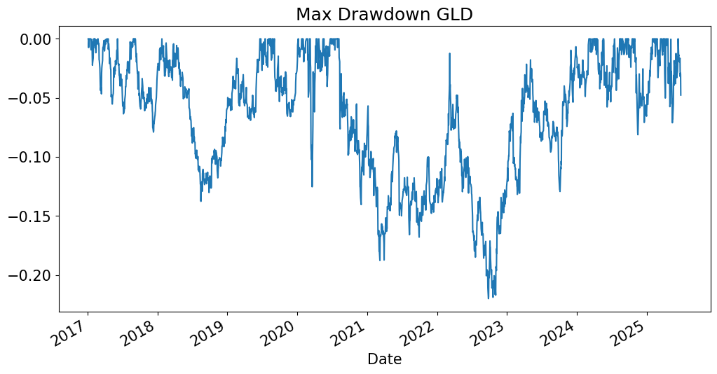
TICK = 'GLD'

drawdown = mdd_timeseries(rets)
drawdown[TICK].plot(title=f'Max Drawdown {TICK}');
plt.show()
tailMetrics(rets,relative=False)[['VaR (0.05)','CVaR (0.05)']].style.format('{:.2%}')
| VaR (0.05) | CVaR (0.05) | |
|---|---|---|
| SPY | -1.76% | -2.90% |
| VEA | -1.57% | -2.56% |
| UPRO | -5.28% | -8.70% |
| GLD | -1.44% | -2.04% |
| USO | -3.54% | -5.93% |
| FXE | -0.73% | -0.96% |
| BTC | -6.25% | -9.80% |
| HYG | -0.71% | -1.27% |
| IEF | -0.68% | -0.95% |
| TIP | -0.53% | -0.86% |
| SHV | -0.02% | -0.03% |
QUANT = .05

quants = rets.quantile(QUANT).to_frame()
quants.columns = [f'quantile {QUANT}']

quants.sort_values(quants.columns[0]).style.format('{:.1%}')
| quantile 0.05 | |
|---|---|
| BTC | -6.2% |
| UPRO | -5.3% |
| USO | -3.5% |
| SPY | -1.8% |
| VEA | -1.6% |
| GLD | -1.4% |
| FXE | -0.7% |
| HYG | -0.7% |
| IEF | -0.7% |
| TIP | -0.5% |
| SHV | -0.0% |
Sampling error in mean#
Given by LLN, diminishes with \(\sqrt{N}\).
mu = rets.mean()
se = rets.std()/np.sqrt(rets.shape[0])
ratio = mu/quants[f'quantile {QUANT}'].values
tab = pd.concat([mu,se,ratio],axis=1)
tab.columns = ['mean','standard error','mean as fraction of quantile']
tab.style.format('{:.2%}')
| mean | standard error | mean as fraction of quantile | |
|---|---|---|---|
| SPY | 0.06% | 0.03% | -3.44% |
| VEA | 0.04% | 0.02% | -2.45% |
| UPRO | 0.15% | 0.08% | -2.92% |
| GLD | 0.05% | 0.02% | -3.55% |
| USO | 0.02% | 0.05% | -0.56% |
| FXE | 0.01% | 0.01% | -0.87% |
| BTC | 0.31% | 0.10% | -5.04% |
| HYG | 0.02% | 0.01% | -2.59% |
| IEF | 0.00% | 0.01% | -0.73% |
| TIP | 0.01% | 0.01% | -2.07% |
| SHV | 0.01% | 0.00% | -47.35% |
2#
# LOADETF = '../data/risk_etf_data.xlsx'
# px = pd.read_excel(LOADETF,sheet_name='prices').set_index('Date').dropna()
# rets = px.pct_change().dropna()
FREQ_LABEL = 'daily'
FREQ_LABEL_AGG = 'monthly'
CODE_RESAMPLE = 'ME'

px = (1+rets).cumprod()
retsM = px.resample(CODE_RESAMPLE).last().pct_change().dropna()
retsM.dropna(inplace=True)
#retsM.tail().style.format('{:.1%}').format_index('{:%Y-%m-%d}')
keyX = 'SPY'
pd.concat([bivariate_risk(rets,keyX=keyX),bivariate_risk(retsM,keyX=keyX)],axis=1,keys=[FREQ_LABEL,'monthly']).style.format('{:.2%}')
| daily | monthly | |||||
|---|---|---|---|---|---|---|
| SPY corr | SPY cov | SPY beta | SPY corr | SPY cov | SPY beta | |
| SPY | 100.00% | 0.01% | 100.00% | 100.00% | 0.21% | 100.00% |
| VEA | 86.51% | 0.01% | 80.34% | 86.69% | 0.18% | 86.13% |
| UPRO | 99.89% | 0.04% | 299.36% | 99.56% | 0.66% | 308.90% |
| GLD | 8.66% | 0.00% | 6.56% | 12.69% | 0.02% | 10.42% |
| USO | 30.10% | 0.01% | 61.63% | 32.62% | 0.17% | 80.14% |
| FXE | 14.17% | 0.00% | 5.54% | 31.23% | 0.03% | 13.60% |
| BTC | 25.09% | 0.01% | 92.96% | 34.22% | 0.37% | 172.43% |
| HYG | 78.16% | 0.01% | 36.00% | 83.25% | 0.09% | 40.88% |
| IEF | -13.15% | -0.00% | -4.80% | 18.70% | 0.02% | 7.90% |
| TIP | 5.96% | 0.00% | 1.90% | 55.73% | 0.04% | 18.40% |
| SHV | -6.19% | -0.00% | -0.09% | 1.89% | 0.00% | 0.07% |
pd.concat([get_moments(rets,doStyle=False),get_moments(retsM,doStyle=False)],axis=1,keys=[FREQ_LABEL,FREQ_LABEL_AGG]).style.format('{:.2f}')
| daily | monthly | |||||||
|---|---|---|---|---|---|---|---|---|
| mean | vol | skewness | kurtosis | mean | vol | skewness | kurtosis | |
| SPY | 0.00 | 0.01 | -0.30 | 14.24 | 0.01 | 0.05 | -0.48 | 0.39 |
| VEA | 0.00 | 0.01 | -0.86 | 16.12 | 0.01 | 0.05 | -0.34 | 1.32 |
| UPRO | 0.00 | 0.04 | -0.38 | 14.99 | 0.03 | 0.14 | -0.53 | 0.94 |
| GLD | 0.00 | 0.01 | -0.15 | 2.70 | 0.01 | 0.04 | 0.43 | -0.30 |
| USO | 0.00 | 0.02 | -1.28 | 16.30 | 0.01 | 0.11 | -1.53 | 7.27 |
| FXE | 0.00 | 0.00 | 0.16 | 1.35 | 0.00 | 0.02 | 0.32 | -0.26 |
| BTC | 0.00 | 0.04 | 0.03 | 6.15 | 0.07 | 0.23 | 0.57 | 0.09 |
| HYG | 0.00 | 0.01 | 0.13 | 26.42 | 0.00 | 0.02 | -0.94 | 4.94 |
| IEF | 0.00 | 0.00 | 0.20 | 3.20 | 0.00 | 0.02 | -0.01 | -0.04 |
| TIP | 0.00 | 0.00 | 0.36 | 14.86 | 0.00 | 0.02 | -0.82 | 3.47 |
| SHV | 0.00 | 0.00 | 0.66 | 3.28 | 0.00 | 0.00 | 0.36 | -1.21 |