TA Review 6 - Factor Pricing and Momentum

Anand Nakhate

Factor Pricing Models

When did our field stop being “asset pricing” and become “asset expected returning?” … Market-to-book ratios should be our left-hand variable, the thing we are trying to explain, not a sorting characteristic for expected returns.

– Cochrane

Factor pricing model vs linear decomposition

Linear factor decomposition (statistical):

• \( r_{i,t} \;=\; \alpha_i \;+\; \boldsymbol{\beta}_i^\top \boldsymbol{f}_t \;+\; \varepsilon_{i,t}, \qquad \mathbb{E}[\varepsilon_{i,t}]=0. \)

• Purely descriptive. Estimates how much variation in \(r_{i,t}\) co‑moves with $boldsymbol{f}_t$.

• No restriction that \(\alpha_i=0\) or that loadings must price expected returns.

• Applications include performance attribution, hedging, tracking etc.

Factor pricing model (economic):

• impose no‑arbitrage via a stochastic discount factor (SDF) \(m_{t+1}\): \( \mathbb{E}\!\left[m_{t+1} R_{i,t+1}\right]=0 \;\; \forall i. \)

• With a linear SDF \(m_{t+1}=a-b^\top \boldsymbol{f}_{t+1}\) and traded factors, this yields beta–lambda pricing: \( \mathbb{E}[r_i] \;=\; \boldsymbol{\beta}_i^\top \boldsymbol{\lambda}, \qquad \boldsymbol{\beta}_i := \frac{\mathrm{Cov}(r_i,\boldsymbol{f})}{\mathrm{Var}(\boldsymbol{f})}, \)

• So correctly specified models imply \(\alpha_i=0\) in the time‑series and risk premia \(\boldsymbol{\lambda}\) explain cross‑sectional mean returns.

A linear decomposition explains variance. A pricing model explains expected returns

Factor Pricing: Expected vs Realized Returns

• In factor pricing models, expected returns are theoretical, forward-looking forecasts based on an asset’s exposure to systematic risk factors, whereas realized returns are the backward-looking, actual historical gains or losses an investor experiences.

• The key difference between the two is the presence of unexpected returns (or “surprises”), which cause realized returns to deviate from their expected values over any given period.

---

Note on Stochastic discount factor:

All asset prices can be written with a stochastic discount factor (SDF) \(m_{t+1}\):

\( P_t=\mathbb{E}_t\!\left[m_{t+1}X_{t+1}\right], \qquad \mathbb{E}_t\!\left[m_{t+1}R_{i,t+1}\right]=1, \)

Economic intuition: in bad states (low aggregate consumption/wealth), marginal utility is high and \(m_{t+1}\) is high. Assets that pay off in bad states hedge investors (high \(\operatorname{Cov}(m,R)\)) and therefore earn low premia. Assets that pay off in good states are cyclical, have negative covariation with \(m\), and must offer high premia.

Empirically, we approximate the SDF with traded or macro factors \(f_{t+1}\):

\( m_{t+1}\approx a - b^{\top} f_{t+1} \;\;\Longrightarrow\;\; \mathbb{E}[R_i^{e}] \approx \beta_i^{\top}\lambda, \qquad \beta_i=\frac{\operatorname{Cov}(R_i,f)}{\operatorname{Var}(f)}. \)

Cyclical equities have high \(\beta\) (they pay in good times when \(m\) is low) and thus higher expected returns. Defensive/hedging assets have low or negative \(\beta\) and lower premia.

\( \boxed{\text{Expected returns = prices of aggregate risks }(\lambda)\times\text{ risk exposures }(\beta).} \)

---

Testing factor pricing models

1.1 Time-Series Test of a Factor Model

A factor pricing model is consistent with the data if each asset’s alpha is statistically indistinguishable from zero. Estimate, for each test asset \(i\), $\( r_{i,t}^e \;=\; \alpha_i \;+\; \beta_i^\top f_t \;+\; \varepsilon_{i,t}, \qquad H_0:\ \alpha_i=0\ \text{(for all \)i\(; joint test).} \)$

What the test asks: Do the factors price assets (no leftover average returns after accounting for factor exposures)?

How to read results.

• If \(\alpha_i\approx 0\) (individually and jointly), the model passes a pricing test.

• We then focus on the \(\beta_i\)’s: once a model is accepted, \(\beta_i\) summarize each asset’s risk profile and are the inputs to expected-return calculations.

• We do not use \(R^2\) here as a success metric. A high time-series \(R^2\) aids replication/hedging, but pricing restricts means (alphas), not variance decompositions.

Significant alphas signal model misspecification (omitted risks, wrong factors, or time-variation not captured). A model with small alphas but modest \(R^2\) can still be an excellent pricing model.

---

1.2 Cross-Sectional Test

Having estimated \(\beta_i\) from the time-series step, test whether differences in average returns are explained by differences in factor exposures. Let \(\bar r_i\) be the sample mean excess return of asset \(i\). Run $\( \bar r_i \;=\; \eta \;+\; \beta_i^1 \lambda_1 \;+\; \beta_i^2 \lambda_2 \;+\;\cdots\;+\; \beta_i^n \lambda_n \;+\; \nu_i, \)$

Interpretation.

• \(\beta_i^k\) are the (estimated) factor loadings. \(\lambda_k\) are prices of risk.

• In a correctly specified model with traded factors, \(\eta\approx 0\) and \(\lambda_k\) align with the factors’ expected excess returns.

• Here, cross-sectional \(R^2\) is informative: higher \(R^2\) means betas explain more of the dispersion in average returns.

Insight & implication.

• Positive \(\lambda_k\) indicates the \(k\)-th risk is rewarded: assets with higher \(\beta_i^k\) should earn higher expected returns.

• Low \(R^2\) or \(\eta\neq 0\) suggests missing factors, measurement error in betas, or instability (time-varying betas/prices of risk).

• The time-series (alphas) and cross-section (risk prices) tests are complementary: passing one does not guarantee passing the other.

---

Factor Test Workflow

1. Estimate \(\beta_i\) via time-series regressions

2. run the cross-sectional regression to estimate \(\boldsymbol\lambda\)

3. use accepted \(\beta\)–\(\lambda\) structure to compute and compare expected returns across assets/portfolios.

---

CAPM (single‑factor) and its limits

Model: $\(\mathbb{E}\left[\tilde{r}^i\right] = \beta^{i,m}\mathbb{E}\left[\tilde{r}^m\right]\)$

LFD: $\( r_{i,t} \;=\; \alpha_i \;+\; \beta_{iM}\, r_{M,t} \;+\; \varepsilon_{i,t}, \quad \mathbb{E}[r_i] = \beta_{iM}\,\lambda_M, \quad \alpha_i=0 \text{ if CAPM holds.} \)$

Predictions: Market beta alone explains expected returns. Alphas are zero for well‑diversified portfolios.

Issues:

• Size, value, profitability/investment, and momentum patterns generate systematic alphas vs CAPM.

• Conditional betas/expected returns vary through time. Single source of risk is too restrictive.

• Low‑risk/low‑beta anomalies (e.g., betting‑against‑beta) contradict linear risk‑return under CAPM.

Test Results:

1. In the time-series, the alphas are considerably large and sometimes statistically significant.

2. In the cross-section, the \(R^2\) is low (25.8% in the sample), indicating that CAPM does not fit the data well.

3. If we allow for a proper cross-sectional regression, \(\lambda_m\) (the market premium) is -0.0982, which contradicts the historical market premium of 0.0802.

CAPM is a useful benchmark but insufficient to price broad cross‑sections.

---

Fama–French 3‑factor model

The expected excess return of any asset is a linear combination of three β’s: Market Factor, Value Factor, Size Factor. It implies that nothing else matters in determining which assets have high mean returns.

• In the rational interpretation, this only holds if investors are risk-averse to these β’s: if they are, the prices of assets with these β’s become smaller, leading to higher expected returns.

• In a behavioral interpretation, investors may be systematically biased against certain characteristics, though not necessarily due to extra risk.

Model: $\( \mathbb{E}\left[\tilde{r}^i\right] = \beta^{i,m}\mathbb{E}\left[\tilde{r}^m\right] + \beta^{i,s}\mathbb{E}\left[\tilde{r}^s\right] + \beta^{i,\nu}\mathbb{E}\left[\tilde{r}^{\nu}\right] \)$

LDF: $\( r_{i,t} \;=\; \alpha_i \;+\; \beta_M r_{M,t} \;+\; \beta_S\, \mathrm{SMB}_t \;+\; \beta_H\, \mathrm{HML}_t \;+\; \varepsilon_{i,t}. \)$

Factor construction: (One Possible way)

• Sort by size (S,B) and book‑to‑market (L,M,H).

• \(\mathrm{SMB} = \tfrac{1}{3}(S/L + S/M + S/H) - \tfrac{1}{3}(B/L + B/M + B/H)\).

• \(\mathrm{HML} = \tfrac{1}{2}(S/H + B/H) - \tfrac{1}{2}(S/L + B/L)\).

Captures size and value premia left unexplained by CAPM. Materially reduces joint test rejections on standard test portfolios.

Note: Factors dont have to be orthogonal. The less multi-collinear the factors are the better statistical power the model has. This has no mathematical or computational benifit

---

Note: Long–short factors: what does this achieve?

Mechanics: Rank stocks on a signal, form quantile portfolios, and take long top – short bottom (e.g., winners–losers, value–growth). Weighting often is value‑ or equal‑weighted. Tebalanced monthly/quarterly with rules to control turnover.

Why long–short?

• Isolates the characteristic while neutralizing market (dollar neutral) exposure (near zero beta by construction).

• Reduces multicollinearity as we hedge out market exposure

• Facilitates clean tests of pricing: TS alphas close to zero under the correct model.

• Improves interpretability: factor returns are pure payoffs to the targeted style, usable in regressions, risk models, and portfolio construction.

Implementation levers: Breadth (universe), weighting (value/equal/risk‑parity), rebalance cadence, signal definitions ( z‑scoring), and constraints (industry/sector neutrality).

---

Fama–French 5‑factor model

\( r_{i,t} \;=\; \alpha_i \;+\; \beta_M r_{M,t} \;+\; \beta_S \mathrm{SMB}_t \;+\; \beta_H \mathrm{HML}_t \;+\; \beta_R \mathrm{RMW}_t \;+\; \beta_C \mathrm{CMA}_t \;+\; \varepsilon_{i,t}. \)

New factors (canonical construction).

• RMW (Robust Minus Weak): high‑profitability minus low‑profitability portfolios.

• CMA (Conservative Minus Aggressive): low investment (asset growth) minus high.

Adding RMW & CMA often shrinks HML’s role (value overlap with profitability/investment). Momentum is not included here—practitioners often add UMD explicitly in “FF5+Mom”.

Fama-French Factor Data: https://mba.tuck.dartmouth.edu/pages/faculty/ken.french/data_library.html

Note:

Factor Model does not mean that value or small stocks have higher mean returns! These factors suggest that stocks with a positive relationship to the factors will have high mean returns. It’s about how the company’s returns behave, not its size or label.

For instance, a stock with a high B/M ratio but behaving like a growth stock will have low expected returns. Conversely, a stock with a low B/M ratio behaving like a value stock will have high expected returns.

The key determinant of expected return is the β, not the stock’s characteristics!

---

Other widely used factors

Though Fama-French improves on CAPM, it still doesn’t capture all systematic risk. Today, there is a proliferation of factors and factor models, often referred to as the ”zoo factor.”

Some common factors used in the industry:

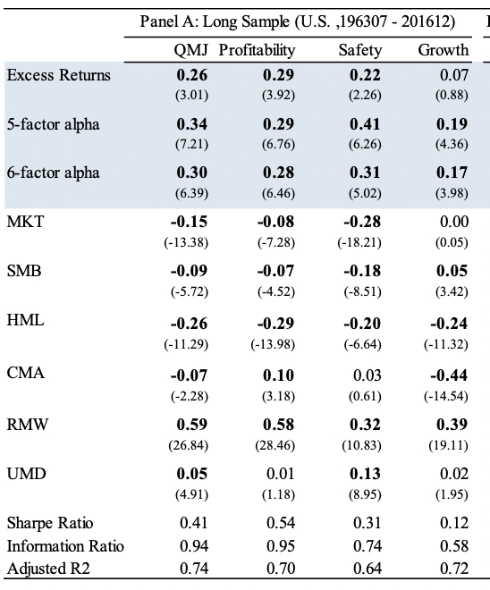
• Quality / QMJ: profitability, growth, safety, payout, often paired with value.

• Low‑risk / BAB: betting‑against‑beta / low‑volatility premia. Linked to leverage constraints and lottery preference.

• Liquidity: exposure to liquidity shocks.

• Carry/Value/Momentum across asset classes (FX, rates, commodities, credit) for multi‑asset diversification.

Treat factors as tradable long–short portfolios for risk modeling and alpha decomposition, or convert to tilts in long‑only mandates with constraints (beta neutrality, sector neutrality, turnover budgets).

A lot of literature exists on various factors. Reference: https://www.openassetpricing.com/

Factor construction

We have looked at long short construction based on ranking. Following are different ways to construct the factors:

(A) Z‑scores & linear‑combination portfolios

• Cross‑sectionally standardize signal \(x_{i,t}\) to \(z_{i,t}=(x_{i,t}-\mu_t)/\sigma_t\).

• Build exposure‑targeting weights via cross‑sectional regression (factor‑mimicking portfolio): \( \min_{\boldsymbol{w}_t}\;\|\boldsymbol{X}_t^\top \boldsymbol{w}_t - \boldsymbol{e}_k\|^2 \quad\text{s.t.}\quad \boldsymbol{1}^\top\boldsymbol{w}_t=0,\; \boldsymbol{\beta}_M^\top \boldsymbol{w}_t=0. \) This yields a portfolio that loads \(+1\) on target signal \(k\), neutral on others/market.

(B) PCA / statistical factors

• Extract latent factors from the covariance of returns: eigen‑portfolios maximize explained variance.

• Good for risk modeling. Not guaranteed to price expected returns without economic backing.

(C) Multi‑signal / composites

• Combine signals via weighting or ridge/lasso on future returns. Stabilize with z‑score averaging:

  \( \text{Composite}_i = \sum_{s=1}^{S} \omega_s\, z_{i}^{(s)}, \quad \sum_s \omega_s=1. \)

---

Is a factor “useful”? Tangency (Sharpe) test and spanning

Let base asset set have mean \(\boldsymbol{\mu}_B\) and covariance \(\Sigma_B\). The max Sharpe (squared) is

\( S^2(\mathcal{B}) \;=\; \boldsymbol{\mu}_B^\top \Sigma_B^{-1} \boldsymbol{\mu}_B. \)

Augment with a candidate factor \(g\) (as a tradable long–short portfolio). Recompute

\( S^2(\mathcal{B}\cup g) \;=\; \boldsymbol{\mu}^\top \Sigma^{-1} \boldsymbol{\mu}. \)

H_0: no improvement, \(S^2(\mathcal{B}\cup g)-S^2(\mathcal{B})=0\) ⇔ spanning holds.

Equivalent regression (spanning form).

\( r_{g,t} \;=\; a \;+\; \boldsymbol{b}^\top \boldsymbol{r}_{B,t} \;+\; \eta_t. \)

• If \(a=0\), \(g\) is spanned by the base set; no Sharpe improvement.

• Evaluate out‑of‑sample Sharpe changes, report turnover, capacity, and drawdown/correlation impacts. Apply deflated Sharpe when selecting among many candidates.

Example: Quality Minus Junk Factor (AQR) - https://www.aqr.com/Insights/Research/Working-Paper/Quality-Minus-Junk

---

Momentum

What is Momentum?

Momentum is nothing but autoregressive effect.

For a broad market index, there is little evidence of strong serial correlation—positive or negative. A simple test regresses next period’s index return on its own lag:

\[ r_{t+1}^m \;=\; \alpha \;+\; \beta\, r_t^m \;+\; \varepsilon_{t+1}. \]

• Typically, \(\beta \approx 0\) and is statistically insignificant; any exploitable serial correlation would be rapidly arbitraged away.

• Even when weak autocorrelation exists, the associated \(R^2\) is small, implying limited economic value and high implementation risk for a pure index-timing rule.

Momentum as a Strategy

If the regression above revealed a small positive \(\beta\), one could translate that intuition to the cross-section by buying recent winners and shorting recent losers—harvesting persistence in relative performance rather than timing the aggregate index.

• Diversifying across many stocks reduces idiosyncratic variance, improving the signal-to-noise ratio even when the edge per name is small.

• Emphasizing extremes (e.g., top vs. bottom quantiles of past returns) amplifies the signal while diversification helps contain volatility.

Key levers for Momentum Strategy

If we have an edge, we can act differently and gain from momentum

• Lever 1: Play on winners and losers, and not just one asset

• Lever 2: Play on a number of winners and losers

• Lever 3: Play with transaction costs. We can do this either by slowing down the ranking (12 months vs 1 month) or increaing the band of winners and losers.

Construction of Cross Sectional Momentum Strategy:

Constructing cross sectinoal momentum: Rank stocks each month by past 12‑month return skipping the most recent month (12–2). Go long top quantile (winners) and short bottom quantile (losers). Rebalance monthly.

UMD / MOM factor (Fama–French data). A standard construction uses top 30% – bottom 30% past‑return portfolios. Momentum has been pervasive across long samples, remains present after the early 1990s academic publication, and shows low correlation to market/size and negative correlation to value—making it a powerful complement to value‑tilted portfolios.

Implementation details.

• Skip month t‑1 to avoid short‑term reversal effects. Rank on \(t-12\) to \(t-2\).

• Use broad, liquid universes. Control for industry tilts or combine with industry momentum.

• Manage turnover and crash risk (e.g., during sharp factor rotations).

Momentum rationales

Risk‑based views.

• Winner portfolios can load on time‑varying macro/volatility/liquidity risks. Momentum legs co‑move strongly, so drawdowns are possible when those risks pay off in reverse.

• Negative correlation with value implies diversifying but sometimes crash‑prone joint dynamics.

Behavioral views.

• Under‑reaction to news -> gradual drift as information is incorporated (post‑earnings announcement drift).

• Over‑reaction / feedback trading -> trend chasing and slow correction.

• Limits to arbitrage (shorting costs, career risk) let patterns persist.

from IPython.display import HTML

with open('../_static/ta_review_momentum/momentum_construction.html', 'r') as f:
    external_html_content = f.read()

HTML(external_html_content)

If the iframe does not load in your Jupyter Book (e.g., due to strict Content Security Policy), you can also open the standalone file at ../_static/ta_review_momentum/momentum_construction.html.

HW 6 - Momentum Strategies

Case Study

In early 2009, AQR considered launching three long‑only, open‑end retail mutual funds to deliver the equity momentum factor to a broad advisor/retail channel—the first retail funds explicitly dedicated to momentum. The strategy is the classic cross‑sectional winner‑minus‑loser effect: stocks that outperformed their peers over the prior 12 months (skipping the most recent month) continue to outperform, and vice versa. The case walks through the empirical evidence, the regulatory and product‑design constraints of retail mutual funds, AQR’s decision to build their own long‑only momentum indices, and the implementation choices (rebalance, trading, taxes, tracking error, and whether to co‑mix other signals).

What AQR is doing?

Product scope: AQR planned three funds aligned to three new long‑only momentum indices:

• US Large‑Cap (top 1,000 US stocks),

• US Small‑Cap (next 2,000),

• International Large‑Cap (~1,000 non‑US large caps).

Constituents were reselected each quarter as the top one‑third of the universe by past t‑12 to t‑2 returns (skipping the last month), and cap‑weighted to avoid unintended small‑cap bets.

Distribution: Unlike AQR’s hedge funds, the target channel here was financial advisors in the retail mutual fund market (open‑end funds with daily NAV and daily liquidity), not institutional LPs.

Index first, fund second. Because mutual fund advisors cannot use backtests, AQR created and licensed momentum indices that could publish historical performance independently of fund marketing. The indices doubled as investor tools and as possible benchmarks for the eventual funds.

Why not simply use UMD?

UMD is long‑short, monthly‑rebalanced, and built from the full stock universe (including microcaps)—not replicable as a retail long‑only fund. Hence AQR created long‑only, large‑ and small‑cap indices with quarterly rebalances and liquidity screens.

The five big implementation choices:

• Rebalance frequency (quarterly vs. more often).

• Boundary (edge) trading.

• Execution speed (fast vs. slow).

• Taxes (very real for retail).

• Should other signals influence buys/sells? (Ex: Short term reversal?)

The hardest empirical nuance: momentum crash risk

Momentum’s long‑run mean is high, but its left tail can be vicious—notably during sharp market rebounds after deep selloffs when past losers rip higher and past winners lag.

Trading costs & capacity—will alpha survive implementation?

AQR’s design choices directly address this:

• Cap‑weighting within the top third avoids oversized micro‑cap exposure.

• Quarterly rebalance + banding reduces unnecessary turnover.

• Large internal flow potential enables crossing and schedule control.

All three raise the odds that net‑of‑cost alpha remains positive in a mutual‑fund wrapper.

1. READING - The Momentum Product

This section is not graded, and you do not need to submit your answers. But you are expected to consider these issues and be ready to discuss them.

1.1

What is novel about the AQR Momentum product under construction compared to the various momentum investment products already offered?

It’s the first retail mutual fund offering dedicated momentum exposure. Momentum had been common in hedge funds and institutional mandates, but not in open‑end mutual funds available via the financial‑adviser channel. To enable retail access, AQR designed long‑only, cap‑weighted momentum indices (large‑cap US, small‑cap US, large‑cap international) rebalanced quarterly, with S&P as calculation agent. This differs from the academic UMD long‑short factor and from monthly all‑stock rebalancing. It also focuses on liquid names to serve daily flows. Mutual Funds also tend to be open-ended - be ready to return capital at the end of the trading day to respond to investor redemptions if any.

1.2

Name three reasons the momentum investment product will not exactly track the momentum index, (ie. why the strategy will have tracking error.)

AQR lists key implementation choices that create tracking error:

(wrt/ AQR Momentum Index):

• Rebalance cadence: the index rebalances quarterly. Trading more/less frequently improves signal freshness or reduces costs, but deviates from index weights.

• Boundary trading: deciding when (or whether) to swap a position moving from rank ~333 to 350 changes holdings vs the ‘top‑third’ cut, causing tracking slippage.

• Execution schedule: fast trading minimizes stale exposure but costs more. Slow trading cuts costs but drifts from index weights.

• Additional TE drivers: tax‑aware trading (harvesting vs index), and minor tilts/timing using additional signals (e.g., short‑term reversal, value).

(wrt/ UMD Index):

• AQR’s fund would be long-only, whereas the index (Fama-french UMD) is long-short.

• The index assumes monthly rebalancing, which may cause huge transaction cost.

• Fama-French UMD used all listed stocks, whereas AQR’s fund would only use stocks with reasonable market capitalization and liquidity. This is because of “open-end” mutual fund regulation.

1.3

When constructing the momentum portfolio, AQR ranks stocks on their returns from month \(t-12\) through \(t-2\). Why don’t they include the \(t-1\) return in this ranking?

Because last‑month returns tend to reverse. Excluding t−1 avoids trading into the short‑term reversal effect (Jegadeesh (1990)).

2. Investigating Momentum

⚠️ IMPORTANT: Data Loading Required

This section requires data that is not included in this notebook. The code cells below will not run as-is.

To run this section, you need to:

1. Download the data file momentum_data.xlsx from Canvas

2. Either:

   • Place it in your current working directory, OR

   • Update the path in the code cell below to point to your data location

The data file should contain momentum factors, decile portfolios, and size-sorted portfolios.

Data

In this section, we empirically investigate some concerns regarding AQR’s new momentum product. On Canvas, find the data file, data/momentum_data.xlsx.

• The first tab contains the momentum factor as an excess return: \(\tilde{r}^{\mathrm{mom}}\).

• The second tab contains returns on portfolios corresponding to scored momentum deciles.

  • \(r^{\operatorname{mom}(1)}\) denotes the portfolio of stocks in the lowest momentum decile, the “losers” with the lowest past returns.

  • \(r^{\operatorname{mom}(10)}\) denotes the portfolio of stocks in the highest momentum decile.

• The third tab gives portfolios sorted by momentum and size.

  • \(r^{\text {momsu }}\) denotes the portfolio of small stocks in the top 3 deciles of momentum scores.

  • \(r^{\text {momBD }}\) denotes the portfolio of big-stocks in the bottom 3 deciles of momentum scores.

Note that the Fama-French momentum return, \(\tilde{r}^{\mathrm{mom}: \mathrm{FF}}\), given in the first tab, is constructed by \(\mathrm{FF}\) as,

\[ \tilde{r}^{\mathrm{mom}: \mathrm{FF}}=\frac{1}{2}\left(r^{\mathrm{momBU}}+r^{\mathrm{momSU}}\right)-\frac{1}{2}\left(r^{\mathrm{momBD}}+r^{\mathrm{momSD}}\right) \]

import pandas as pd, numpy as np
from pathlib import Path
from datetime import datetime
import matplotlib.pyplot as plt
import seaborn as sns

# UPDATE THIS PATH: Point to where you saved momentum_data.xlsx
# Option 1: If in current directory
xlsx_path = Path('momentum_data.xlsx')
# Option 2: If in data subfolder
# xlsx_path = Path('../data/momentum_data.xlsx')
# Option 3: Use absolute path
# xlsx_path = Path('/Users/yourname/path/to/momentum_data.xlsx')

xls = pd.ExcelFile(xlsx_path)

desc      = pd.read_excel(xls, 'descriptions')
mom_ex    = pd.read_excel(xls, 'momentum (excess returns)')
factors   = pd.read_excel(xls, 'factors (excess returns)')
deciles   = pd.read_excel(xls, 'deciles (total returns)')
size_tot  = pd.read_excel(xls, 'size_sorts (total returns)')
rf_df     = pd.read_excel(xls, 'risk-free rate')

for df in [mom_ex, factors, deciles, size_tot, rf_df]:
    df['Date'] = pd.to_datetime(df['Date'])
    df.set_index('Date', inplace=True)
    df.sort_index(inplace=True)

mom_ex.tail()

	UMD
Date
2025-04-30	0.0497
2025-05-31	0.0221
2025-06-30	-0.0264
2025-07-31	-0.0096
2025-08-31	-0.0354

The Fama-French momentum return

\[\tilde{r}^{mom:FF} = \frac{1}{2} (\tilde{r}^{momBU} + \tilde{r}^{momSU}) − \frac{1}{2} (\tilde{r}^{momBD} + \tilde{r}^{momSD}) \]

size_tot = size_tot.join(rf_df, how='inner')
for col in ['SMALL LoPRIOR','SMALL HiPRIOR','BIG LoPRIOR','BIG HiPRIOR']:
    size_tot[f'EX_{col}'] = size_tot[col] - size_tot['RF'] 

FF_MOM_excess = 0.5*(size_tot['EX_SMALL HiPRIOR'] + size_tot['EX_BIG HiPRIOR']) \
              - 0.5*(size_tot['EX_SMALL LoPRIOR'] + size_tot['EX_BIG LoPRIOR'])
FF_MOM_excess.name = 'FF_MOM_excess'
FF_MOM_excess.to_frame().tail()

	FF_MOM_excess
Date
2025-04-30	0.04975
2025-05-31	0.02215
2025-06-30	-0.02635
2025-07-31	-0.00965
2025-08-31	-0.03540

FF_MOM_longonly_excess = 0.5*(size_tot['EX_SMALL HiPRIOR'] + size_tot['EX_BIG HiPRIOR'])
FF_MOM_longonly_excess.name = 'FF_MOM_longonly_excess'
FF_MOM_longonly_excess.to_frame().tail()

	FF_MOM_longonly_excess
Date
2025-04-30	-0.00070
2025-05-31	0.06925
2025-06-30	0.04265
2025-07-31	0.00210
2025-08-31	0.03160

factors = pd.DataFrame({'UMD': mom_ex['UMD']}) \
    .join(factors[['MKT','SMB', 'HML']], how='inner') \
    .join(pd.DataFrame({'FF_MOM': FF_MOM_excess,
                        'FF_MOM_longonly': FF_MOM_longonly_excess,
                        'RF': rf_df['RF']}), how='inner')

factors.tail()

	UMD	MKT	SMB	HML	FF_MOM	FF_MOM_longonly	RF
Date
2025-04-30	0.0497	-0.0084	-0.0059	-0.0340	0.04975	-0.00070	0.0035
2025-05-31	0.0221	0.0606	0.0070	-0.0288	0.02215	0.06925	0.0038
2025-06-30	-0.0264	0.0486	0.0083	-0.0160	-0.02635	0.04265	0.0034
2025-07-31	-0.0096	0.0198	0.0027	-0.0127	-0.00965	0.00210	0.0034
2025-08-31	-0.0354	0.0185	0.0387	0.0441	-0.03540	0.03160	0.0038

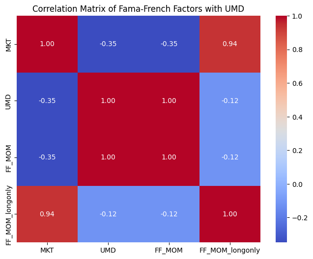
# Plot Correlation Matrix:

corr = factors[["UMD", "HML", "MKT", "SMB"]].corr()
plt.figure(figsize=(8,6))
sns.heatmap(corr, annot=True, fmt=".2f", cmap='coolwarm')
plt.title('Correlation Matrix of Fama-French Factors with UMD')
plt.show()

# Momentum Correlation Matrix:
import matplotlib.pyplot as plt
import seaborn as sns
corr = factors[["MKT", "UMD", "FF_MOM", "FF_MOM_longonly"]].corr()
plt.figure(figsize=(8,6))
sns.heatmap(corr, annot=True, fmt=".2f", cmap='coolwarm')
plt.title('Correlation Matrix of Fama-French Factors with UMD')
plt.show()

2.1 Is Momentum sill profitable?

The excess returns of lucrative trading strategies often disappear once the strategy is well-known. The first widely-cited paper on momentum was published in 1993. Have momentum returns or risk changed since then? The AQR case takes place at the end of 2008. Have momentum returns changed in 2009-2024?

Investigate by filling out the summary statistics below for the full-sample and three sub-samples.

(a)

Using the data provided, fill in Table 1 with the appropriate stats for \(\tilde{r}^{\text {mom:FF }}\).

\[\begin{split} \begin{equation*} \begin{aligned} &\text { Table 2: Long-only momentum performance. }\\ &\begin{array}{llllll} \hline \hline \text { Subsample } \quad \text { mean } \quad \text { vol } & \text { Sharpe } & \text { skewness } & \text { corr. to } \tilde{r}^m & \text { corr. to } \tilde{r}^v \\ \hline \hline & & & & \\ 1927-2024 & & & \\ 1927-1993 & & & \\ 1993-2008 & & & \\ 2009-2024 & & & \\ \hline \hline \end{array} \end{aligned} \end{equation*} \end{split}\]

series = factors['UMD']
cuts = {
    '1927–2024': (pd.Timestamp('1927-01-31'), pd.Timestamp('2024-12-31')),
    '1927–1993': (pd.Timestamp('1927-01-31'), pd.Timestamp('1993-12-31')),
    '1993–2008': (pd.Timestamp('1993-01-31'), pd.Timestamp('2008-12-31')),
    '2009–2024': (pd.Timestamp('2009-01-31'), pd.Timestamp('2024-12-31')),
}

def stats(x):
    m = float(x.mean()); v = float(x.std(ddof=1))
    return pd.Series({'mean_m': m, 
                      'vol_m': v, 
                      'Sharpe_m': (m/v) if v!=0 else np.nan, 
                      'skewness': float(x.skew()),
                      'kurtosis': float(x.kurtosis())})

table1 = pd.concat({k: stats(series.loc[start:end].dropna()) for k,(start,end) in cuts.items()}, axis=1).T
table1

	mean_m	vol_m	Sharpe_m	skewness	kurtosis
1927–2024	0.006156	0.046970	0.131070	-3.067270	27.984310
1927–1993	0.007345	0.046336	0.158508	-3.911021	38.185026
1993–2008	0.009115	0.049565	0.183901	-0.630596	5.252348
2009–2024	-0.001074	0.045603	-0.023550	-2.691572	16.720118

• UMD average returns are slightly larger post‑1992 (1993–2008)

• Strong positive mean, high volatility, left‑tail risk

• Momentum crashes cluster in violent rebounds after deep selloffs (e.g., 2009, covid). Risk is partly forecastable. Scaling exposure when crash risk is high reduces drawdowns.

(b)

Has momentum changed much over time, as seen through these subsample statistics?

It doesn’t change much in the most of the periods. But the momentum is showing negative return after 2009. It is reasonable stable between 1927 and 2008, and has been slightly negative since 2009.

(c)

Does this data support AQR’s argument that momentum is an important piece of the ideal portfolio? What if mean returns to momentum are in actuality near zero due to transaction costs - would there still be evidence here that momentum is valuable?

long‑short momentum’s mean appears lower post‑2009 with negative skew intact and corr(MOM, HML) < 0, supporting the case’s story that MOM diversifies value even if mean is muted. The case documents near‑zero corr to market and negative corr to HML over 1927–2008. Our post‑2009 line continues to show low market correlation and negative value correlation.

2.2. Whether a long-only implementation of momentum is valuable.

Construct your own long-only implementation:

\[\tilde{r}^{momU:FF} = \frac{1}{2} (\tilde{r}^{momBU} + \tilde{r}^{momSU}) − r^f \]

Note that this is following the FF approach of treating big and small stocks separately. This would be very similar to a scaled version of,

\[\tilde{r}^{momU} = \frac{1}{3} (\tilde{r}^{mom(8)} + \tilde{r}^{mom(9)} + \tilde{r}^{mom(10)}) − r^f \]

For the question below, use the FF-style \(\tilde{r}^{momU:FF}_t\)

(a)

Fill out Table 2 for the data in the period 1994-2024.

\[\begin{split} \begin{equation*} \begin{aligned} &\text { Table 2: Long-only momentum performance. }\\ &\begin{array}{llllll} \hline \hline \text { 1994-2024 } & \text { mean } \quad \text { vol } & \text { Sharpe } & \text { skew } & \text { corr. to } \tilde{r}^m & \text { corr. to } \tilde{r}^v \\ \hline \hline \text { Long-and-short, }\left(\tilde{r}^{\text {mom:FF }}\right) & & & \\ \text { Long-only }\left(\tilde{r}^{\text {momU:FF }}\right) & & & \\ \hline \hline \end{array} \end{aligned} \end{equation*} \end{split}\]

sub = factors.loc['1994-01-31':'2024-12-31']

def stats_with_corr(x, mkt, hml):
    m = float(x.mean()); v = float(x.std(ddof=1))
    return pd.Series({'mean_m': m, 
                      'vol_m': v, 
                      'Sharpe_m': (m/v) if v!=0 else np.nan,
                      'skewness': float(x.skew()),
                      'kurtosis': float(x.kurtosis()),
                      'corr_MKT': float(x.corr(mkt)), 
                      'corr_HML': float(x.corr(hml))})

table2 = pd.DataFrame({
    'Long–Short UMD': stats_with_corr(sub['FF_MOM'], sub['MKT'], sub['HML']),
    'Long–Only UMD': stats_with_corr(sub['FF_MOM_longonly'], sub['MKT'], sub['HML'])
}).T
table2

	mean_m	vol_m	Sharpe_m	skewness	kurtosis	corr_MKT	corr_HML
Long–Short UMD	0.003585	0.048279	0.074263	-1.461204	9.984761	-0.310502	-0.210385
Long–Only UMD	0.009675	0.051371	0.188340	-0.441967	1.155302	0.903985	-0.116289

• Long‑only momentum often has higher market beta and higher correlation to the market (it’s long equities only), so it behaves more like a return booster than a pure diversifier.

• Diversification versus value shrinks somewhat (less negative HML corr than long‑short), but the alpha from the winner leg is still meaningful.

(b)

Is long-only momentum as attractive as long-short momentum with respect to mean, volatility, and Sharpe Ratio?

Yes, long-only looks even more attractive than long-short momentum. The mean return is higher, while the volatility is similar. Sharpe ratio is higher as well.

(c)

Is long-only momentum as diversifying as long-short momentum with respect to market and value premia?

Long‑only momentum typically shows high market correlation (≈0.9) because we keep the “UP” leg without shorting “DOWN”. Long‑short UMD remains low/negative corr to MKT and negative to HML, delivering diversification even when mean returns are low. This is exactly why AQR framed momentum as a complementary style to value. In retail mutual funds, long‑only is the feasible packaging, but its portfolio role is different. It is more return‑seeking, less diversifying.

(d)

Show a plot of the cumulative product of \(1+\tilde{r}^{\text {mom:FF }}\) and \(1+\tilde{r}^{\text {momU:FF }}\) over the 1994-2024 subsample. \(^2\)

sub = factors.loc['1994-01-31':'2024-12-31']
cum_ls  = (1 + sub['FF_MOM']).dropna().cumprod()
cum_lon = (1 + sub['FF_MOM_longonly']).dropna().cumprod()
cum_mkt = (1 + sub['MKT']).dropna().cumprod()

plt.figure(figsize=(9,5))
plt.plot(cum_ls.index,  cum_ls.values,  label='Long–Short (FF_MOM)')
plt.plot(cum_lon.index, cum_lon.values, label='Long–Only (FF_MOM_longonly)')
plt.plot(cum_mkt.index, cum_mkt.values, label='Market (MKT)')
plt.yscale('log')
plt.title('Cumulative Wealth (log scale): Momentum, 1994–2024')
plt.xlabel('Date')
plt.ylabel('Growth of $1')
plt.legend()
plt.tight_layout()

2.3. Is momentum just data mining, or is it a robust strategy?

Assess how sensitive the threshold for the “winners” and “losers” is in the results. Specifically, we compare three constructions:

• long the top 1 decile and short the bottom 1 deciles:

\[ \tilde{r}^{momD1} = r^{mom(10)} - r^{mom(1)}\]

• long the top 3 deciles and short the bottom 3 deciles:

\[\begin{split} \begin{aligned} \tilde{r}^{momD3} &= \frac{1}{3}(r^{mom(8)} + r^{mom(9)} + r^{mom(10)}) - \frac{1}{3} (r^{mom(3)} + r^{mom(2)} + r^{mom(1)})\\ &= \frac{1}{3}\sum_{k = 8}^{10} r^{mom(k)} - \frac{1}{3}\sum_{k = 1}^{3} r^{mom(k)} \end{aligned}\end{split}\]

• long the top 5 deciles and short the bottom 5 decile:

\[ \tilde{r}^{momD5} = \frac{1}{5}\sum_{k = 6}^{10} r^{mom(k)} - \frac{1}{5}\sum_{k = 1}^{5} r^{mom(k)} \]

D = deciles.loc['1994-01-31':'2024-12-31'].copy().dropna()
F = factors.loc['1994-01-31':'2024-12-31'].copy().dropna()
D.columns = ['D1','D2','D3','D4','D5','D6','D7','D8','D9','D10']

rmomD1 = D['D10'] - D['D1']
rmomD3 = D[['D8','D9','D10']].mean(axis=1) - D[['D1','D2','D3']].mean(axis=1)
rmomD5 = D[['D6','D7','D8','D9','D10']].mean(axis=1) - D[['D1','D2','D3','D4','D5']].mean(axis=1)

(a)

Compare all three constructions, (in the full-sample period,) by filling out the stats in the table below for the period 1994-2023.

\[\begin{split} \begin{equation} \begin{aligned} &\text { Table 3: Robustness of momentum construction. }\\ &\begin{array}{lllllll} \hline \hline \text { 1994-2024 } \quad \text { mean } & \text { vol } & \text { Sharpe } & \text { skewness } & \text { corr. to } \tilde{r}^m & \text { corr. to } \tilde{r}^v \\ \hline \hline \tilde{r}^{\text {momD1 }} & & & & & \\ \tilde{r}^{\text {momD3 }} & & & & \\ \tilde{r}^{\text {momD5 }} & & & & \\ \hline \hline \end{array} \end{aligned} \end{equation} \end{split}\]

def stats_corr(x, mkt, hml):
    m = float(x.mean()); v = float(x.std(ddof=1))
    return pd.Series({'mean_m': m, 'vol_m': v, 'Sharpe_m': (m/v) if v!=0 else np.nan,
                      'skewness': float(x.skew()),
                      'corr_MKT': float(x.corr(mkt.loc[x.index])),
                      'corr_HML': float(x.corr(hml.loc[x.index]))})
table3 = pd.DataFrame({
    'rmomD1 (10–1)': stats_corr(rmomD1, F['MKT'], F['HML']),
    'rmomD3 (avg 8–10 minus 1–3)': stats_corr(rmomD3, F['MKT'], F['HML']),
    'rmomD5 (avg 6–10 minus 1–5)': stats_corr(rmomD5, F['MKT'], F['HML']),
    'mom': stats_corr(F['FF_MOM'], F['MKT'], F['HML']),
}).T
table3

	mean_m	vol_m	Sharpe_m	skewness	corr_MKT	corr_HML
rmomD1 (10–1)	0.006748	0.086474	0.078037	-1.301211	-0.324182	-0.237460
rmomD3 (avg 8–10 minus 1–3)	0.002478	0.055908	0.044325	-1.341123	-0.363161	-0.212109
rmomD5 (avg 6–10 minus 1–5)	0.001438	0.038763	0.037106	-1.421454	-0.354419	-0.208658
mom	0.003585	0.048279	0.074263	-1.461204	-0.310502	-0.210385

• Robustness supports AQR’s “top third” (broad winners) choice—implementation matters more than squeezing the last basis point from a fragile threshold.

(b)

Do the tradeoffs between the 1-decile, 3-decile, and 5-decile constructions line up with the theoretical tradeoffs we discussed in the lecture?

Yes, we can see long-short portfolio with higher threshold of decile has higher return, but also higher volatility.

(c)

Should AQR’s retail product consider using a 1-decile or 5-decile construction?

I would recommend 1-decile, as it has higher sharpe, but can also see the argument for a 5 decile construction due to likely lower turnover (and therefore lower fees for investors).

(d)

Does \(\tilde{r}^{\text {momD3 }}\) have similar stats to the Fama-French construction in (1). Recall that construction is also a 3-decile, long-short construction, but it is segmented for small and large stocks. Compare the middle row of Table 3 with the top row of Table 2.

The signal is robust to “reasonable” winner/loser set choices. D1 has the highest Sharpe but the highest volatility and turnover. D3 and D5 are smoother, more capacity‑friendly (fits a mutual‑fund wrapper). Our D3 row should look similar in spirit to FF’s MOM (both are 3‑decile long‑short constructs, though FF splits by size), consistent with the case that the phenomenon is broad and not a narrow parameter pick.

2.4.

Does implementing momentum require trading lots of small stocks– thus causing even larger trading costs?

For regulatory and liquidity reasons, AQR is particularly interested in using larger stocks for their momentum baskets. (Though they will launch one product that focuses on medium-sized stocks.)

Use the data provided on both small-stock “winners”, \(r^{momSU}\), and small-stock “losers”, \(r^{momSD}\), to construct a small-stock momentum portfolio,

\[ r^{momS}_t = r^{momSU}_t - r^{momSD}_t \]

Similarly, use the data provided to construct a big-stock momentum portfolio,

\[ r^{momB}_t = r^{momBU}_t − r^{momBD}_t \]

S = size_tot.loc['1994-01-31':'2024-12-31'].copy().dropna()
F = factors.loc['1994-01-31':'2024-12-31'].copy().dropna()
S.columns = ["SL", "SM", "SH", "BL", "BM", "BH", "RF", "ESL", "ESH", "EBL", "EBH"]

(a)

Fill out Table 4 over the sample 1994-2024.

\[\begin{split} \begin{equation*} \begin{aligned} &\text { Table 4: Momentum of small and big stocks. }\\ &\begin{array}{llllll} \hline \hline \text { 1994-2024 } & \text { mean } & \text { vol } & \text { Sharpe } & \text { skewness } & \text { corr. to } \tilde{r}[m] \\ \hline \hline \text { All stocks, } \tilde{r}^{\text {mom:FF }} & & & & \\ \text { Small stocks } r_t^{\text {mom } S} & & & \\ \text { Large stocks } r_t^{\text {mom } B} & & & \\ \hline \end{array} \end{aligned} \end{equation*} \end{split}\]

rmomS = S["SH"] - S["SL"]
rmomB = S["BH"] - S["BL"]


table4 = pd.DataFrame({
    'rmomS (SH–SL)': stats_corr(rmomS, F['MKT'], F['HML']),
    'rmomB (BH–BL)': stats_corr(rmomB, F['MKT'], F['HML']),
    'mom': stats_corr(F['FF_MOM'], F['MKT'], F['HML']),
}).T
table4

	mean_m	vol_m	Sharpe_m	skewness	corr_MKT	corr_HML
rmomS (SH–SL)	0.005118	0.048828	0.104812	-1.804211	-0.310223	-0.139319
rmomB (BH–BL)	0.002053	0.052628	0.039009	-0.874482	-0.281863	-0.256739
mom	0.003585	0.048279	0.074263	-1.461204	-0.310502	-0.210385

• Large‑cap momentum is cleaner and more scalable (fits retail flows and daily cash).

• Small‑cap momentum adds alpha. design features (cap‑weighting, quarterly rebalance, buffers) are crucial to keep slippage, and transaction costs in check.

(b)

Is the attractiveness of the momentum strategy mostly driven by the small stocks? That is, does a momentum strategy in large stocks still deliver excess returns at comparable risk? We’ll typically see both small and big momentum show positive mean with negative corr to HML, but small‑stock momentum is noisier and costlier to trade. That’s why AQR built a large‑cap momentum index with cap‑weighting and quarterly rebalance—to ensure capacity and lower slippage for an open‑end retail fund

2.5.

In conclusion, what is your assessment of the AQR retail product? Is it capturing the important features of the Fama-French construction of momentum? Would you suggest any modifications?

• UMD is a monthly, long–short, all‑stocks, frictionless backtest. Its lifetime properties (low market corr, negative HML corr, sizable mean) are precisely why it’s an orthogonal return source in multi‑factor portfolios.

• AQR Momentum: Retail packaging forces long‑only, cap‑weighted, liquidity‑filtered, quarterly rebalances — a different factor. We expect high market beta and therefore different portfolio role. It is a return booster rather than diversifier.

• AQR’s retail product uses a long only approach which leads to a higher correlation with the Market and has less diversification benefits compared to the benchmark index or Fama-French momentum factor.

• Quarterly rebalancing might make the portfolio diverge from the benchmark index and Fama-French momentum factor.

• Risk/vol management overlay. Combine with value for better diversification

• Tax‑aware trading: Harvest losses on the fly, and defer gains into long‑term buckets

• Cross‑asset extension

Case Study - “Fact, Fiction, and Momentum Investing,”

Reference: https://www.aqr.com/Insights/Research/Journal-Article/Fact-Fiction-and-Momentum-Investing

The authors set out to debunk 10 persistent myths about cross‑sectional momentum—i.e., buying recent relative winners and selling recent relative losers (12‑month return skipping the most recent month, the canonical “12–2” signal). They use Kenneth French’s public factor library and a stack of peer‑reviewed studies (including their own) to show that momentum is

• (i) large,

• (ii) implementable long‑only or long–short,

• (iii) works in large caps as well as small,

• (iv) survives costs and taxes, and

• (v) is best combined with value.

Factors & construction.

• RMRF (market), SMB (size), HML (value), UMD (momentum: top 30% prior 12–1 winners minus bottom 30% losers, size‑balanced). Definitions mirror French’s library.

• They examine long‑short spread returns, Sharpe ratios, hit ratios (percent positive over rolling horizons), and long vs. short leg contributions (market‑adjusted alphas for winners and losers separately).

Myth 1. “Momentum returns are too small and sporadic.” — False. (HW6)

• Magnitude & Sharpe: UMD shows an annualized spread of ~8.3% (1927–2013) with Sharpe ~0.50, larger than HML (~4.7%, Sharpe ~0.39) and SMB (~2.9%, Sharpe ~0.26).

• Consistency. Rolling 1‑yr hit ratio for UMD is ~81% (1927–2013), and 5‑yr hit ~88%—best or tied‑best across factors.

Momentum is not “sporadic” by any portfolio‑level metric. Its long‑term Sharpe and hit ratios are top‑tier.

Myth 2. “Momentum only works on the short side.” — False. (HW6)

• Long vs. short contributions: Over 1927–2013, winners (long leg) contribute ~5.5% and losers (short leg) contribute ~5.1% (market‑adjusted), roughly half each of the UMD premium.

• On a simple return‑minus‑market view, the long leg accounts for ~74% of UMD (6.1% of 8.3%).

Long‑only investors can capture a meaningful momentum premium by overweighting winners/underweighting losers relative to cap‑weight.

Myth 3. “Momentum exists only in small caps.” — False (HW6)

• Large vs. small: Momentum is strong in large caps (e.g., ~6.8% p.a. 1927–2013) and stronger in small, but the drop‑off to large caps is smaller than for value, which is robust in small caps and weak to non‑existent in large caps over several windows.

If we run large‑cap equity, momentum is the sturdier style than pure book‑to‑price value.

Myth 4. “Momentum doesn’t survive trading costs.” — False

• Using >$1T of live trades (1998–2013) across 19 DM equity markets, per‑dollar costs are low and patient execution, and modest tracking‑error allowances preserve the premium.

• Prior papers overstate costs by using average market costs rather than large‑manager costs and by ignoring cost‑aware portfolio design.

Institutional scale, and patient execution = implementable momentum.

Myth 5. “Momentum is tax‑inefficient because of turnover.” — False / nuanced.

• Despite higher turnover, momentum holds winners (defer gains), sells losers (realize short‑term losses), and has low dividend exposure.

• Value is the opposite on dividends.

• Net: similar tax burden to value, and tax‑aware timing (e.g., one‑month delays to reach long‑term gains) improves momentum more than value.

Myth 6. “Use momentum only as a screen, not a factor.” — False.

• Once we accept momentum’s efficacy, using it directly in optimization dominates using it as a “screen after value.”

• Empirically, factor‑based portfolio construction beats screen‑based approaches.

Myth 7. “Momentum will disappear now that it’s known.” — No evidence of decay. (HW6)

• Out‑of‑sample (post‑1991), momentum did not weaken despite lower trading costs and growth of arbitrage capital.

• Even in the extreme thought experiment where expected UMD return = 0, its diversification with value (corr ≈ −0.4) makes the optimal weight still positive.

Myth 8. “Momentum is too volatile / crash‑prone to rely on.” — Context matters.

• 2009 momentum “crashes” when sharp rebounds after deep bear markets torched the short‑leg (losers) as high‑beta laggards ripped.

• The long leg did fine.

• A simple beta‑hedge or pairing with value mitigates these episodes

• The 60/40 HML/UMD combination shows much smaller drawdowns (worst ≈ −30%) than either alone (value ≈ −43%, momentum ≈ −77%).

Myth 9. “Different momentum definitions give different answers—so it’s unstable.” — Misleading.

• Multiple reasonable definitions work

• 12–1 (skip month 1) is a simple, robust default.

• Over long spans, alternative windows (e.g., 7–12 vs. 1–6 months) converge, and combining measures can help—exactly as with value

Myth 10. “There is no theory.” — There are risk‑based and behavioral theories, and both can imply persistence. (HW6)

• Behavioral: underreaction, and occasional overreaction/feedback.

• Risk‑based: cash‑flow/discount‑rate risks tied to investment/growth options - common cross‑asset “momentum” risk.

• Practically, whichever mix is “true,” persistence follows if the underlying frictions or priced risks persist.

Important Conclusion:

• Combine momentum with value. The two have strong negative correlation (≈ −0.4 in French’s data) and complementary drawdown profiles.

• A 60/40 HML/UMD blend delivers a Sharpe ~0.80, with ~81% positive 1‑yr and ~92% positive 5‑yr rolling windows over 1927–2013.

• You get higher risk‑adjusted returns, fewer and smaller tail events, and better out‑of‑sample reliability than either factor alone.

Case Study — “Value & Momentum Everywhere”

Reference: https://www.aqr.com/Insights/Research/Journal-Article/Value-and-Momentum-Everywhere

Value and Momentum are pervasive across major asset classes and negatively correlated with each other. A simple 50/50 Value–Momentum mix delivers strong, stable risk‑adjusted returns and underpins a global three‑factor model alongside the market. Funding‑liquidity risk helps explain opposite‑signed exposures of Value vs Momentum. Macro exposures are weak.

Motivation for this paper:

• Are Value and Momentum just factors of U.S. equities, or global risk premia that appear everywhere?

• Do these premia co‑move across otherwise unrelated markets?

• Can a simple global factor model price a broad cross‑section spanning multiple asset classes?

Data Universe: Eight diverse markets/asset classes. The study spans individual equities (U.S., U.K., Europe, Japan), country equity index futures, sovereign bonds, currencies, and commodity futures. Methods and return construction are harmonized across assets.

Signals and Factor construction

Momentum \(MOM_{2–12}\)

\(\text{MOM}_{i,t-1} \;=\; \frac{P_{i,t-1}}{P_{i,t-12}} - 1,\quad \text{skip the most recent month.}\)

Skipping one month avoids short‑term reversal/microstructure effects.

Value

For equities: book‑to‑market (BE/ME)

For other assets (where BE/ME is not defined), we use simple, analogous valuation or long‑run price‑based proxies to maintain cross‑asset consistency.

Rank‑weighted long–short factors (per asset class, per date)

Let \(S_{i,t-1}\in\{\text{VAL},\text{MOM}\}\) be the signal for asset \(i\).

Define ranks within a date and center them:

\(w_{i,t-1}\;=\;\frac{\mathrm{rank}(S_{i,t-1})-\overline{\mathrm{rank}}_t}{\sum_j \left|\mathrm{rank}(S_{j,t-1})-\overline{\mathrm{rank}}_t\right|/2}, \qquad \sum_i w_{i,t-1}=0,\quad \sum_{i:w>0} w_{i,t-1}\approx 1,\;\sum_{i:w<0} w_{i,t-1}\approx -1.\)

The factor return next period: \(r_t^{S} \;=\; \sum_i w_{i,t-1}\,R_{i,t}, \quad S\in\{\text{VAL},\text{MOM}\}.\)

Combination: \(r^{\text{COMBO}}_t \;=\; \tfrac{1}{2}\,r^{\text{VAL}}_t \;+\; \tfrac{1}{2}\,r^{\text{MOM}}_t.\)

Cross‑asset aggregation:

Within each asset class: form \(r^{\text{VAL}}_t\) and \(r^{\text{MOM}}_t\) as above. Across classes: combine sleeves with comparable risk (e.g., equal‑volatility weights) to construct VAL_everywhere and MOM_everywhere.

Testing the ideas:

1. Return premia — Show that Value, Momentum, and 50/50 Combo deliver economically and statistically strong returns within each asset class and globally

2. Correlation structure — Document that Value correlates positively with Value across assets, Momentum with Momentum across assets, but Value vs Momentum is strongly negative within and across assets

3. Global factor model — Show that a three‑factor model \([\,\text{MKT},\,\text{VAL\_EW},\,\text{MOM\_EW}\,]\) prices a broad set of global test assets and even FF U.S. portfolios and hedge‑fund indices

Findings

• Universality: Value and Momentum premia exist in every asset class examined.

• Correlation structure is the edge: Value–Value and Momentum–Momentum are positively correlated across assets. Value vs Momentum is strongly negative within and across assets. Styles act like global factors. This could imply we should always combine Value and Momentum (50/50) — diversification is structural, not incidental.

• 50/50 dominates: Because both premia are positive on average and negatively correlated, a simple equal‑weight mix improves Sharpe and stability everywhere. This implies that the 50/50 sleeve is a natural core allocation.

• A practical model: A global three‑factor model \([\,\text{MKT}, \text{VAL\_EW}, \text{MOM\_EW}\,]\) prices a broad set of assets and many equity portfolios. This is useful for risk attribution, budgeting, and hedge‑fund replication.