Exercise - Replicating Regressions

Exercise - Replicating Regressions#

Data#

Use the file, data/port_decomp_example.xlsx.

The data file contains…

Return rates, $r_t^i$, for various asset classes, (via ETFs.)
Most notable among these securities is SPY, the return on the S&P 500. Denote this as $r^{\spy}_t$.
A separate tab gives return rates for a particular portfolio, $r_t^p$.

\[\newcommand{\spy}{\text{spy}}\]

\[\newcommand{\hyg}{\text{hyg}}\]

\[\newcommand{\targ}{EEM}\]

1. Decomposition#

1. Single Factor Exposure#

Estimate the regression of the portfolio return on SPY:

\[r^p_t = \alpha + \beta r^{\spy}_t + \epsilon_t^{p,\spy}\]

Specifically, report your estimates of alpha, beta, and the r-squared.

2. Multi-factor Exposure#

Estimate the regression of the portfolio return on SPY and on HYG, the return on high-yield corporate bonds, denoted as $r^{\hyg}_t$:

\[r^p_t = {\alpha} + {\beta}^{\spy}r^{\spy}_t + {\beta}^{\hyg}r^{\hyg}_t + {\epsilon}_t\]

Specifically, report your estimates of alpha, the betas, and the r-squared.

*Note that the parameters (such as $\beta^{\spy}$) in this multivariate model are not the same as used in the univariate model of part 1.

3. Replication Values#

Calculate the series of fitted regression values, sometimes referred to as $\hat{y}$ in standard textbooks:

\[\hat{r}^p_t = \hat{\alpha} + \hat{\beta}^{\spy}r^{\spy}_t + \hat{\beta}^{\hyg}r^{\hyg}_t\]

Your statistical package will output these fitted values for you, or you can construct them using the estimated parameters.

How does this compare to the r-squared of the regression in problem 2?

4. Uni vs Multi#

How do the SPY betas differ across the univariate and multivariate models? How does this relate to the correlation between $r^{\spy}$ and $r^{\hyg}$?

Solution 1#

import pandas as pd
import numpy as np
import statsmodels.api as sm
from sklearn.linear_model import LinearRegression
from matplotlib import pyplot as plt

INFILE = "../data/assignment_2_data.xlsx"
info = pd.read_excel(INFILE,sheet_name='descriptions').set_index('ticker')
info

	shortName	quoteType	currency	volume	totalAssets	longBusinessSummary
ticker
SPY	SPDR S&P 500	ETF	USD	25604208	627773800448	The Trust seeks to achieve its investment obje...
EFA	iShares MSCI EAFE ETF	ETF	USD	10653257	54985711616	The fund generally will invest at least 80% of...
EEM	iShares MSCI Emerging Index Fun	ETF	USD	17962107	17468592128	The fund generally will invest at least 80% of...
PSP	Invesco Global Listed Private E	ETF	USD	8928	277930496	The fund generally will invest at least 90% of...
QAI	NYLI Hedge Multi-Strategy Track	ETF	USD	49257	637390272	The fund is a "fund of funds" which means it i...
HYG	iShares iBoxx $ High Yield Corp	ETF	USD	22374708	15881510912	The underlying index is a rules-based index co...
DBC	Invesco DB Commodity Index Trac	ETF	USD	478168	1387142912	The fund pursues its investment objective by i...
IYR	iShares U.S. Real Estate ETF	ETF	USD	2699001	4990495744	The fund seeks to track the investment results...
IEF	iShares 7-10 Year Treasury Bond	ETF	USD	2340833	32854654976	The underlying index measures the performance ...
BWX	SPDR Bloomberg International Tr	ETF	USD	180426	959621824	The fund generally invests substantially all, ...
TIP	iShares TIPS Bond ETF	ETF	USD	2132017	15497157632	The index tracks the performance of inflation-...
SHV	iShares Short Treasury Bond ETF	ETF	USD	1850899	18620065792	The fund will invest at least 80% of its asset...

rets = pd.read_excel(INFILE,sheet_name='total returns').set_index('Date')
rets

	BWX	DBC	EEM	EFA	HYG	IEF	IYR	PSP	QAI	SHV	SPY	TIP
Date
2015-02-28	-0.010834	0.044253	0.044080	0.063378	0.022312	-0.024717	-0.025976	0.064102	0.034138	0.000181	0.056204	-0.012886
2015-03-31	-0.013922	-0.060539	-0.014973	-0.014286	-0.009478	0.008561	0.010745	-0.010454	-0.001667	-0.000091	-0.015706	-0.004819
2015-04-30	0.019579	0.071471	0.068527	0.036466	0.008714	-0.006330	-0.048160	0.053982	0.002004	0.000091	0.009834	0.006779
2015-05-31	-0.032312	-0.031711	-0.041045	0.001955	0.003555	-0.004164	-0.003311	0.026868	-0.000333	0.000000	0.012856	-0.010056
2015-06-30	-0.007442	0.016375	-0.029309	-0.031182	-0.018871	-0.016309	-0.043979	-0.019153	-0.013671	0.000091	-0.020312	-0.010246
...	...	...	...	...	...	...	...	...	...	...	...	...
2024-08-31	0.030519	-0.020815	0.009779	0.032603	0.015474	0.013458	0.054008	0.001225	0.007648	0.004979	0.023366	0.007990
2024-09-30	0.023484	0.007237	0.057413	0.007833	0.016971	0.013825	0.030631	0.051617	0.014548	0.004586	0.021005	0.014976
2024-10-31	-0.048497	0.014369	-0.030746	-0.052732	-0.009636	-0.033874	-0.034947	-0.013779	-0.005923	0.003576	-0.008924	-0.018469
2024-11-30	0.002212	-0.019920	-0.026772	-0.003156	0.016446	0.010209	0.040688	0.064952	0.022891	0.003697	0.059633	0.004981
2024-12-31	-0.032164	0.011994	-0.013676	-0.029502	-0.012152	-0.023790	-0.090579	-0.053956	-0.016640	0.000161	-0.020497	-0.017664

119 rows × 12 columns

port =  pd.read_excel(INFILE,sheet_name='portfolio returns').set_index('Date')
port

	portfolio
Date
2015-02-28	0.011887
2015-03-31	0.001796
2015-04-30	0.000374
2015-05-31	0.004765
2015-06-30	-0.023278
...	...
2024-08-31	0.019085
2024-09-30	0.027655
2024-10-31	-0.022130
2024-11-30	0.034685
2024-12-31	-0.046241

119 rows × 1 columns

1.1#

X = sm.add_constant(rets['SPY'])
y = port
mod = sm.OLS(y, X).fit()
mod.summary()

OLS Regression Results
Dep. Variable:	portfolio	R-squared:	0.780
Model:	OLS	Adj. R-squared:	0.778
Method:	Least Squares	F-statistic:	414.7
Date:	Tue, 07 Jan 2025	Prob (F-statistic):	2.86e-40
Time:	16:34:05	Log-Likelihood:	329.70
No. Observations:	119	AIC:	-655.4
Df Residuals:	117	BIC:	-649.8
Df Model:	1
Covariance Type:	nonrobust

	coef	std err	t	P>\|t\|	[0.025	0.975]
const	-0.0034	0.001	-2.332	0.021	-0.006	-0.001
SPY	0.6474	0.032	20.365	0.000	0.584	0.710

Omnibus:	3.740	Durbin-Watson:	1.968
Prob(Omnibus):	0.154	Jarque-Bera (JB):	3.181
Skew:	0.314	Prob(JB):	0.204
Kurtosis:	3.497	Cond. No.	22.7

Notes:
[1] Standard Errors assume that the covariance matrix of the errors is correctly specified.

1.2#

X = sm.add_constant(rets[['SPY', 'HYG']])
y = port
mod_multi = sm.OLS(y, X).fit()
mod_multi.summary()

OLS Regression Results
Dep. Variable:	portfolio	R-squared:	0.825
Model:	OLS	Adj. R-squared:	0.822
Method:	Least Squares	F-statistic:	274.1
Date:	Tue, 07 Jan 2025	Prob (F-statistic):	1.10e-44
Time:	16:34:05	Log-Likelihood:	343.45
No. Observations:	119	AIC:	-680.9
Df Residuals:	116	BIC:	-672.6
Df Model:	2
Covariance Type:	nonrobust

	coef	std err	t	P>\|t\|	[0.025	0.975]
const	-0.0027	0.001	-2.051	0.043	-0.005	-9.11e-05
SPY	0.4241	0.050	8.549	0.000	0.326	0.522
HYG	0.5404	0.098	5.492	0.000	0.346	0.735

Omnibus:	0.907	Durbin-Watson:	2.253
Prob(Omnibus):	0.635	Jarque-Bera (JB):	0.879
Skew:	0.204	Prob(JB):	0.644
Kurtosis:	2.898	Cond. No.	85.4

Notes:
[1] Standard Errors assume that the covariance matrix of the errors is correctly specified.

Notice that the beta on SPY is much lower now that we include HYG. Also note that the R-squared is a little higher.

1.3.#

The squared correlation is exactly the R^2, as R^2 captures the correlation of Portfolio’s return and the combined space spanned by both regressors.

corr_port = port.corrwith(mod.fittedvalues).iloc[0]
corr_port_multi = port.corrwith(mod_multi.fittedvalues).iloc[0]
print(f'Correlation between portfolio and replication: {corr_port_multi:.2%}.')
print(f'Square of this correaltion is {corr_port_multi**2:.2%}\nwhich equals the R-squared.')

Correlation between portfolio and replication: 90.85%.
Square of this correaltion is 82.54%
which equals the R-squared.

1.4.#

TICKreg1 = 'SPY'
TICKreg2 = 'HYG'
corrREGS = rets[TICKreg2].corr(rets[TICKreg1])
print(f'Correlation between {TICKreg1} and {TICKreg2} is {corrREGS:.1%}')

Correlation between SPY and HYG is 81.9%

The beta for SPY in (2) is much smaller than in (1). This is because HYG and SPY are significantly correlated, therefore a large proportion of the variation in the Portfolio return which was being attributed to SPY (in eq 1) was actually better explained by HYG. Thus, in eq (2) this gets attributed more directly to HYG, and less is attributed to SPY.

2. Portfolio Decomposition#

1. Decompose portfolio holdings#

The portfolio return, $r_t^p$, is a combination of the base assets that are provided here. Use linear regression to uncover which weights were used in constructing the portfolio.

\[r_t^p = \alpha +\left(\boldsymbol{\beta}\right)' \boldsymbol{r}_t + \epsilon_t\]

where $\boldsymbol{r}$ denotes the vector of returns for the individual securities.

What does the regression find were the original weights?
How precise is the estimation? Consider the R-squared and t-stats.

Feel free to include an $\alpha$ in this model, even though you know the portfolio is an exact function of the individual securities. The estimation should find $\alpha$ of (nearly) zero.

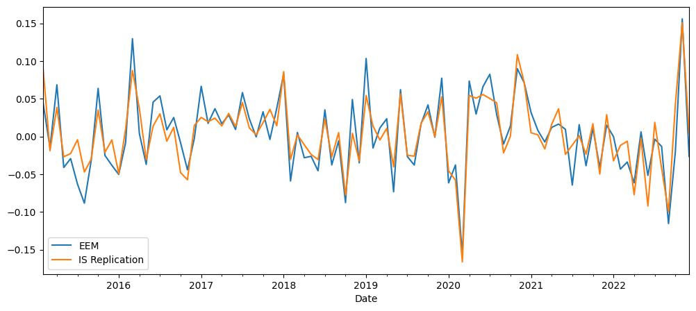
2. Replicate an asset#

Suppose that we want to mimic a return, EEM using the other returns. Run the following regression–but do so only using data through the end of 2022.

\[r_t^{\targ} = \alpha +\left(\boldsymbol{\beta}^{\boldsymbol{r}}\right)' \boldsymbol{r}_t + \epsilon_t\]

where $\boldsymbol{r}$ denotes the vector of returns for the other securities, excluding the target, EEM.

(a)#

Report the r-squared and the estimate of the vector, $\boldsymbol{\beta}$.

(b)#

Report the t-stats of the explanatory returns. Which have absolute value greater than 2?

(c)#

Plot the returns of EEM along with the replication values.

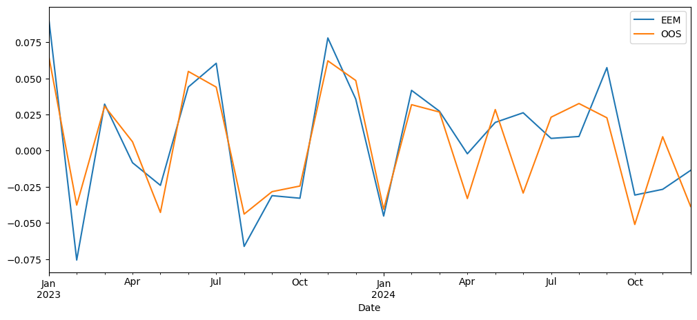
3. Out-of-Sample Fit#

Perhaps the replication results in the previous problem are overstated given that they estimated the parameters within a sample and then evaluated how well the result fit in the same sample. This is known as in-sample fit.

Using the estimates through 2022, (the α and βˆ from the previous problem,) calculate the out-of-sample (OOS) values of the replication, using the 2023-2024 returns, denoted $\boldsymbol{r}_t^{\text{oos}}$:

\[\hat{r}_t^{\targ} = \left(\widehat{\boldsymbol{\beta}}^{\boldsymbol{r}}\right)' \boldsymbol{r}_t^{\text{oos}}\]

(a)#

What is the correlation between $\hat{r}_t^{\targ}$ and $\boldsymbol{r}_t^{\text{oos}}$?

(b)#

How does this compare to the r-squared from the regression above based on in-sample data, (through 2022?)

Solution 2#

2.1#

X = sm.add_constant(rets)
y = port
mod_exact = sm.OLS(y, X).fit()
display(mod_exact.params.to_frame().rename(columns={0:'weights'}).sort_values('weights',ascending=False).T.style.format('{:.2f}'))
mod_exact.summary()

	IYR	PSP	QAI	IEF	SHV	EEM	EFA	HYG	const	BWX	DBC	SPY	TIP
weights	0.25	0.25	0.25	0.25	0.00	0.00	0.00	0.00	0.00	0.00	0.00	0.00	-0.00

OLS Regression Results
Dep. Variable:	portfolio	R-squared:	1.000
Model:	OLS	Adj. R-squared:	1.000
Method:	Least Squares	F-statistic:	1.685e+29
Date:	Tue, 07 Jan 2025	Prob (F-statistic):	0.00
Time:	16:34:05	Log-Likelihood:	4114.2
No. Observations:	119	AIC:	-8202.
Df Residuals:	106	BIC:	-8166.
Df Model:	12
Covariance Type:	nonrobust

	coef	std err	t	P>\|t\|	[0.025	0.975]
const	1.735e-16	3.3e-17	5.259	0.000	1.08e-16	2.39e-16
BWX	1.665e-16	2.13e-15	0.078	0.938	-4.05e-15	4.39e-15
DBC	6.939e-18	6.74e-16	0.010	0.992	-1.33e-15	1.34e-15
EEM	7.008e-16	9.75e-16	0.719	0.474	-1.23e-15	2.63e-15
EFA	3.634e-16	1.57e-15	0.232	0.817	-2.74e-15	3.47e-15
HYG	2.776e-16	2.28e-15	0.122	0.903	-4.25e-15	4.8e-15
IEF	0.2500	3e-15	8.34e+13	0.000	0.250	0.250
IYR	0.2500	8.33e-16	3e+14	0.000	0.250	0.250
PSP	0.2500	1.08e-15	2.31e+14	0.000	0.250	0.250
QAI	0.2500	5.36e-15	4.66e+13	0.000	0.250	0.250
SHV	1.11e-15	1.58e-14	0.070	0.944	-3.02e-14	3.24e-14
SPY	0	1.56e-15	0	1.000	-3.1e-15	3.1e-15
TIP	-1.665e-16	3.8e-15	-0.044	0.965	-7.69e-15	7.36e-15

Omnibus:	17.654	Durbin-Watson:	0.719
Prob(Omnibus):	0.000	Jarque-Bera (JB):	38.094
Skew:	0.563	Prob(JB):	5.35e-09
Kurtosis:	5.533	Cond. No.	702.

Notes:
[1] Standard Errors assume that the covariance matrix of the errors is correctly specified.

2.2#

T1 = '2022'
T2 = '2023'
TICKrep = 'EEM'

rets_IS = rets.loc[:T1,:]

X = sm.add_constant(rets_IS.drop(columns=TICKrep))
y = rets_IS[[TICKrep]]
mod_replicate = sm.OLS(y, X).fit()
mod_replicate.summary()

OLS Regression Results
Dep. Variable:	EEM	R-squared:	0.789
Model:	OLS	Adj. R-squared:	0.761
Method:	Least Squares	F-statistic:	28.25
Date:	Tue, 07 Jan 2025	Prob (F-statistic):	1.50e-23
Time:	16:34:05	Log-Likelihood:	221.60
No. Observations:	95	AIC:	-419.2
Df Residuals:	83	BIC:	-388.6
Df Model:	11
Covariance Type:	nonrobust

	coef	std err	t	P>\|t\|	[0.025	0.975]
const	0.0045	0.004	1.231	0.222	-0.003	0.012
BWX	0.8016	0.218	3.682	0.000	0.369	1.235
DBC	-0.0003	0.073	-0.004	0.997	-0.145	0.144
EFA	0.5235	0.184	2.844	0.006	0.157	0.890
HYG	-0.2021	0.237	-0.853	0.396	-0.673	0.269
IEF	-0.8203	0.350	-2.343	0.022	-1.517	-0.124
IYR	-0.0130	0.094	-0.139	0.890	-0.200	0.173
PSP	-0.1470	0.142	-1.038	0.302	-0.429	0.135
QAI	1.9912	0.560	3.558	0.001	0.878	3.104
SHV	-2.1211	3.064	-0.692	0.491	-8.215	3.973
SPY	-0.2012	0.183	-1.098	0.275	-0.566	0.163
TIP	0.2022	0.431	0.469	0.640	-0.656	1.060

Omnibus:	1.305	Durbin-Watson:	2.314
Prob(Omnibus):	0.521	Jarque-Bera (JB):	1.215
Skew:	-0.272	Prob(JB):	0.545
Kurtosis:	2.895	Cond. No.	1.19e+03

Notes:
[1] Standard Errors assume that the covariance matrix of the errors is correctly specified.
[2] The condition number is large, 1.19e+03. This might indicate that there are
strong multicollinearity or other numerical problems.

The R-squared is reported in the table above.#

Note that while we can estimate an R-squared, it doesn’t make much sense in a regression without an intercept.

It does not need to be between 0 and 1.

The stats-models Python package puts a “Note” at the bottom of the table above reminding users of that fact.

See the t-stats below, in descending order:#

mod_replicate.tvalues.sort_values(ascending=False).to_frame().rename(columns={0:'t-stats'}).T.style.format('{:.1f}')

	BWX	QAI	EFA	const	TIP	DBC	IYR	SHV	HYG	PSP	SPY	IEF
t-stats	3.7	3.6	2.8	1.2	0.5	-0.0	-0.1	-0.7	-0.9	-1.0	-1.1	-2.3

pd.concat([y, mod_replicate.fittedvalues.rename('IS Replication')], axis=1).plot(figsize=(12, 5))
plt.show()

../_images/a8c4e06a6246eab7534d78fd50249ae6f168d65185024ce479b2284ddf132348.png

2.3#

reg = LinearRegression(fit_intercept=True).fit(X,y)
fit_comp_IS = pd.concat([y,pd.DataFrame(reg.predict(X),index=y.index)],axis=1).rename(columns={0:'IS'})
corr_IS = fit_comp_IS.corr().iloc[0,1]

rets_OOS = rets.loc[T2:,:]
X = sm.add_constant(rets_OOS.drop(columns=TICKrep))
y = rets_OOS[[TICKrep]]

fit_comp_OOS = pd.concat([y,pd.DataFrame(reg.predict(X),index=y.index)],axis=1).rename(columns={0:'OOS'})
corr_OOS = fit_comp_OOS.corr().iloc[0,1]

print(f'Correlation between {TICKrep} and Replicating Portfolio')
print(f'In-Sample: {corr_IS:.1%}')
print(f'Out-of-Sample: {corr_OOS:.1%}')

Correlation between EEM and Replicating Portfolio
In-Sample: 88.8%
Out-of-Sample: 85.0%

fit_comp_OOS.plot(figsize=(12, 5))
plt.show()

../_images/99230f851c3b2087492dd14f3ca9885adf2b92a0c5b7dd9956acb384099455cc.png

Exercise - Replicating Regressions

Contents

Exercise - Replicating Regressions#

Data#

1. Decomposition#

1. Single Factor Exposure#

2. Multi-factor Exposure#

3. Replication Values#

4. Uni vs Multi#

Solution 1#

1.1#

1.2#

1.3.#

1.4.#

2. Portfolio Decomposition#

1. Decompose portfolio holdings#

2. Replicate an asset#

(a)#

(b)#

(c)#

3. Out-of-Sample Fit#

(a)#

(b)#

Solution 2#

2.1#

2.2#

The R-squared is reported in the table above.#

See the t-stats below, in descending order:#

2.3#