P.2 Managing Tail Risk#
Project Statement#
In March 2020, portfolio volatility exploded overnight and backward-looking VaR models were immediately obsolete. In 2022, volatility rose only modestly—yet a standard 60/40 portfolio had its worst year in decades, because stocks and bonds fell together. These are fundamentally different failures: one is a volatility shock, the other is a correlation shock.
Your task is to build, compare, and stress-test VaR models for a multi-asset portfolio, then test whether the same methods survive contact with concentrated single-stock risk. You will work with 5% VaR throughout, comparing methods that differ in their distributional assumptions, their volatility dynamics, and whether they model assets individually or jointly. The goal is not just to find the “best” model, but to understand which dimension of the model fails first in different regimes—and what happens when the diversification that portfolio VaR relies on disappears entirely.
Context#
VaR as a Two-Dimensional Problem#
A VaR estimate involves two independent choices:
How do you estimate volatility? Do you weight all historical data equally (rolling window), or give more weight to recent observations (EWMA)? In Exercise 3.1, you saw that rolling-window VaR adapts slowly to changing conditions. EWMA (\(\lambda = 0.94\)) responds within days.
What distribution do you assume? Given a volatility estimate \(\hat{\sigma}_t\), the Normal distribution converts it to VaR via \(\mu + z_\alpha \hat{\sigma}_t\). But returns have fat tails—the Student-t distribution captures this with a degrees-of-freedom parameter \(\nu\). And one can avoid parametric assumptions entirely by working with the empirical distribution of (appropriately scaled) historical returns.
From Scalar to Multivariate#
The methods above all treat the portfolio as a single return series—they are scalar methods. But a portfolio is a weighted combination of assets, each with their own dynamics and correlations. When correlations shift (as SPY-IEF did in 2022), a scalar model captures this only implicitly.
Monte Carlo simulation models the joint distribution directly: simulate correlated asset returns from an estimated covariance matrix, compute portfolio P&L for each draw, and read off the quantile. This is the industry-standard approach at bank trading desks (Basel FRTB), and it opens the door to risk decomposition and CVaR.
CVaR (Expected Shortfall)#
VaR answers: “What’s the worst loss at the 95th percentile?” But it says nothing about what happens in the remaining 5% of cases. CVaR (Conditional VaR, also called Expected Shortfall) is the average loss given that VaR has been breached:
CVaR is coherent (satisfies subadditivity, unlike VaR) and is the basis for market risk capital under Basel III. Monte Carlo gives CVaR for free—it’s just the mean of the simulated losses in the tail.
Resources#
Course Materials#
Discussion 3.1: Value-at-Risk — Normal VaR, EWMA volatility, historical simulation, backtesting
Exercise 3.1: VaR of Equity Portfolio — Empirical VaR/CVaR, rolling volatility, hit-ratio backtest
Discussion 1.2 — Diversification and correlation
Data#
File |
Description |
Frequency |
Date Range |
|---|---|---|---|
|
Prices for SPY, IEF, GLD, HYG (and others) |
Daily |
2017–2025 |
|
Daily prices and earnings announcement flags for individual stocks |
Daily |
2015–2025 |
The ETF data provides ~2,130 daily observations for the multi-asset portfolio in Q1–Q6. The single-stock file provides data for Q7: the prices sheet contains daily adjusted close prices; the earnings sheet has a binary flag (1/0) indicating the trading day on which each stock’s quarterly earnings result was first reflected in the price (i.e., the first trading day after the after-close announcement).
Data Preview#
import pandas as pd
import numpy as np
import matplotlib.pyplot as plt

DATA_PATH = '../../data/'

prices = pd.read_excel(DATA_PATH + 'risk_etf_data.xlsx', sheet_name='prices',
                       index_col=0, parse_dates=True)
rets = prices.pct_change().dropna()

UNIVERSE = ['SPY', 'IEF', 'GLD', 'HYG']
rets_u = rets[UNIVERSE]

print(f'Daily returns: {rets_u.shape[0]} days, {rets_u.shape[1]} assets')
print(f'Date range: {rets_u.index.min().date()} to {rets_u.index.max().date()}')
rets_u.describe().round(4)
Daily returns: 2132 days, 4 assets
Date range: 2017-01-04 to 2025-06-27
| SPY | IEF | GLD | HYG | |
|---|---|---|---|---|
| count | 2132.0000 | 2132.0000 | 2132.0000 | 2132.0000 |
| mean | 0.0006 | 0.0000 | 0.0005 | 0.0002 |
| std | 0.0119 | 0.0043 | 0.0090 | 0.0055 |
| min | -0.1094 | -0.0251 | -0.0537 | -0.0550 |
| 25% | -0.0037 | -0.0024 | -0.0045 | -0.0017 |
| 50% | 0.0007 | 0.0001 | 0.0006 | 0.0003 |
| 75% | 0.0062 | 0.0025 | 0.0053 | 0.0022 |
| max | 0.1050 | 0.0264 | 0.0485 | 0.0655 |
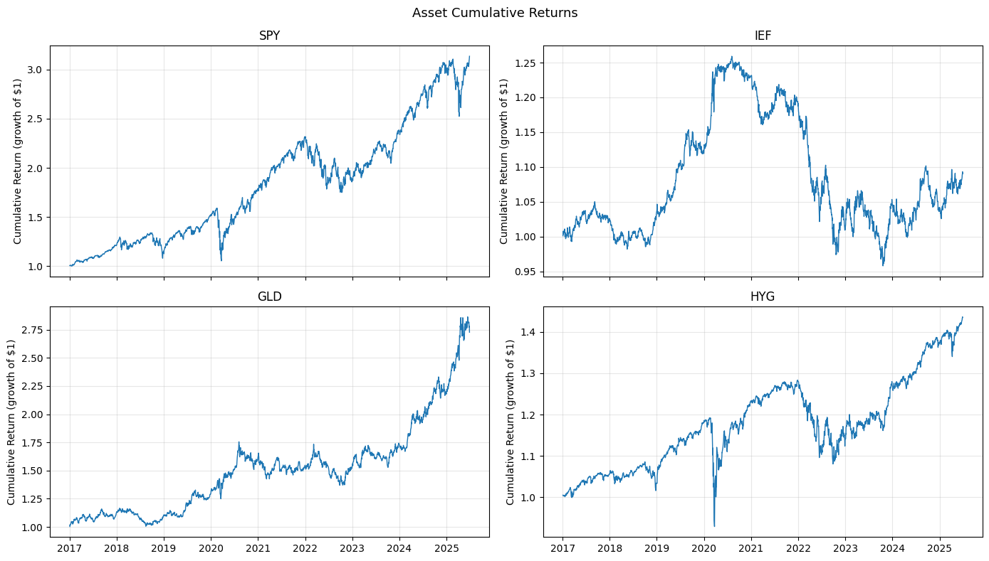
fig, axes = plt.subplots(2, 2, figsize=(14, 8), sharex=True)

for ax, col in zip(axes.flat, UNIVERSE):
    cum = (1 + rets_u[col]).cumprod()
    ax.plot(cum.index, cum, linewidth=1)
    ax.set_title(col)
    ax.set_ylabel('Cumulative Return (growth of $1)')
    ax.grid(True, alpha=0.3)

plt.suptitle('Asset Cumulative Returns', fontsize=13)
plt.tight_layout()
plt.show()
Questions#
Q1: Portfolio Construction and Baseline Risk#
Construct a portfolio from the four ETFs with the following weights:
Asset |
Weight |
Role |
|---|---|---|
SPY |
50% |
Core equity |
IEF |
25% |
Duration / diversifier |
GLD |
10% |
Alternative |
HYG |
15% |
Credit income |
Compute daily portfolio returns and report unconditional summary statistics: annualized mean and volatility, skewness, kurtosis, 5% VaR, and 5% CVaR.
Compare the portfolio’s unconditional 5% VaR to the weighted sum of individual asset VaRs. How large is the diversification benefit? Is there reason to think this benefit is stable over time?
Fit a Student-t distribution to the portfolio returns (e.g., via scipy.stats.t.fit). What degrees of freedom does MLE imply? At the 5% quantile, which distribution—Normal or Student-t—produces a more conservative (larger in magnitude) VaR estimate?
Q2: Time-Varying Volatility and VaR Estimation#
In Exercise 3.1, you backtested VaR using rolling-window volatility and found that it adapts slowly to regime changes. For this project, use EWMA (\(\lambda = 0.94\)) as the volatility model throughout.
Implement the following three scalar VaR methods, each at the 5% level:
Normal + EWMA: \(\text{VaR}_t = \hat{\mu}_t + z_{0.05} \cdot \hat{\sigma}_{\text{EWMA},t}\)
Student-t + EWMA: Replace the Normal quantile \(z_{0.05}\) with the Student-t quantile \(t_{0.05, \nu}\). Use the degrees of freedom from your fit in Q1. Be careful with how the t-distribution’s variance (\(\nu / (\nu-2)\)) interacts with \(\hat{\sigma}_{\text{EWMA}}\): EWMA estimates the actual return variance, but the standard Student-t distribution has variance \(\nu/(\nu-2) \neq 1\), so the quantile must be rescaled to match the EWMA volatility.
Filtered Historical Simulation (FHS): This is a semi-parametric method that combines EWMA dynamics with the empirical distribution. At each date \(t\), take a trailing window of historical returns (e.g., 252 days). Scale each historical return \(r_s\) by the ratio of current to historical EWMA vol: \(\tilde{r}_s = r_s \cdot \hat{\sigma}_t / \hat{\sigma}_s\). The VaR is the 5th percentile of these scaled returns. The idea: EWMA handles the level of volatility, while the historical distribution handles the shape—no need to assume Normal or Student-t.
Plot all three VaR estimates alongside realized portfolio returns. Where do they diverge most?
Q2 Part B (New): GARCH Volatility#
EWMA fixes \(\lambda = 0.94\) by convention. GARCH(1,1) estimates the persistence and shock-response parameters from data:
where \(\omega > 0\), \(\alpha \geq 0\), \(\beta \geq 0\), and \(\alpha + \beta < 1\) for stationarity. Note that EWMA is the special case where \(\alpha + \beta = 1\)—there is no mean-reversion. When \(\alpha + \beta < 1\), the process reverts to a long-run variance \(\bar{\sigma}^2 = \omega / (1 - \alpha - \beta)\). When the fitted persistence is at or very near 1.0, this is called IGARCH—discuss what that implies.
Fit a GARCH(1,1) model to two return series using the arch package (mean = constant, innovation distribution = Normal):
The portfolio return series from Q1.
SPY alone.
For each fit:
Report the estimated parameters (\(\hat{\omega}\), \(\hat{\alpha}\), \(\hat{\beta}\)) and the persistence \(\hat{\alpha} + \hat{\beta}\).
If persistence is below 1, compute the implied long-run annualized volatility. If it equals 1 (IGARCH), explain why the model collapsed to this boundary.
Compare the fitted \(\hat{\alpha}\) to EWMA’s implicit value of \(1 - \lambda = 0.06\). What does a higher \(\hat{\alpha}\) mean for how quickly the model reacts to a large return shock?
Plot the GARCH conditional volatility alongside the EWMA volatility. Where do they diverge most?
Do the two series tell the same story? Why might a diversified portfolio and a single equity produce different GARCH fits — and what does that say about when GARCH adds value beyond EWMA?
Hint: the arch package uses the convention \(r_t = \mu + \varepsilon_t\) where \(\varepsilon_t = \sigma_t z_t\). The fit() method returns the conditional volatility series directly via results.conditional_volatility. Scale your returns to percentage units (multiply by 100) before fitting to avoid numerical issues with very small variances.
Q3: Backtesting#
A well-calibrated 5% VaR should be exceeded on roughly 5% of days. The hit ratio is the fraction of days where the realized return falls below the VaR forecast:
Hit ratio \(\approx\) 5%: well-calibrated
Hit ratio \(\gg\) 5%: model underestimates risk
Hit ratio \(\ll\) 5%: model is too conservative
Compute the hit ratio for each of your three methods over the full sample. Then break it down into at least three sub-periods: pre-COVID (through end of 2019), 2020 (the volatility shock), and 2021–present. If you see evidence that a method’s performance varies within one of these windows, split further—the goal is to identify regime-dependent failures, not to report a single average.
Which methods stay close to 5% across regimes? Are there periods where a method that looks good overall actually fails badly? In your sub-period analysis, look for cases where a method appears well-calibrated in aggregate but fails locally—with exceedances concentrated in a short window rather than spread evenly.
Also examine exceedance clustering: what is the longest streak of consecutive VaR breaches for each method? A model can have the right hit ratio on average but miss badly in concentrated bursts—hit ratio alone cannot detect this.
Q4: Correlation Breakdown#
The three methods in Q2 all operate on the portfolio return series directly—they never model individual assets or their correlations. But correlation instability is a major source of risk model failure.
Compute rolling correlations (e.g., 126-day window) for key asset pairs, especially SPY–IEF. Document the regime shift: when does SPY–IEF turn from negative to positive? How does this relate to the Fed hiking cycle?
To assess the impact on VaR, compare two covariance-based approaches:
Fixed correlation: Use each asset’s EWMA volatility but hold the correlation matrix fixed at its full-sample value.
Rolling covariance: Use a trailing window to estimate the full covariance matrix, updating both volatilities and correlations.
Convert both to a 5% Normal VaR (using \(w'\Sigma w\) for portfolio variance). Compare hit ratios. Does updating correlations help, particularly during 2022?
This comparison motivates the question: if scalar VaR only captures correlation changes implicitly (through the portfolio return itself), can we do better by modeling the joint distribution directly?
Q5: Monte Carlo VaR and CVaR#
Implement a multivariate Monte Carlo VaR. At each date \(t\):
Estimate the mean vector \(\mu\) and covariance matrix \(\Sigma\) from a trailing window of asset returns.
Draw a large number of simulated return vectors from the multivariate Normal distribution \(N(\mu, \Sigma)\).
For each draw, compute the portfolio return \(r_p = w' \cdot r_{\text{sim}}\).
The VaR is the 5th percentile of the simulated portfolio returns. The CVaR is the mean of the simulated returns below the VaR.
You will need to make implementation choices: the covariance estimation window, the number of simulations (1,000–10,000 is typically sufficient for a stable 5th percentile), and how to handle numerical issues. Discuss your choices.
Compare the MC VaR’s hit ratio to the scalar methods from Q2. For a linear portfolio under multivariate Normal assumptions, do you expect MC to produce very different results from Normal+EWMA? Why or why not?
Now compare CVaR across all methods. For the parametric methods, the Normal CVaR has a closed-form expression:
where \(\phi\) is the standard Normal PDF and \(z_\alpha = \Phi^{-1}(\alpha)\). For FHS, the CVaR is simply the mean of the scaled returns that fall below the VaR threshold.
On days when VaR is breached, how does each method’s CVaR forecast compare to the actual average loss? Which methods underestimate the severity of tail losses?
Q5 Part B (New): Factor Decomposition and Systematic Stress Testing#
Your Monte Carlo in Q5 draws from a covariance matrix \(\Sigma\) estimated directly from asset returns. But \(\Sigma\) mixes two distinct sources of risk. Using the linear factor decomposition from Discussion 2.1, regress each asset’s returns on the market factor (SPY):
This is not a CAPM test—we are using the market as a statistical factor to decompose return variation, not making a pricing claim. The decomposition splits each asset’s return into a systematic component (\(\beta_i r_m\)) and an idiosyncratic component (\(\varepsilon_i\)). The covariance matrix of asset returns can then be written:
where \(\beta\) is the vector of factor loadings, \(\sigma_m^2\) is the market variance, and \(D\) is a diagonal matrix of idiosyncratic variances \(\sigma^2_{\varepsilon_i}\).
a) Estimate \(\beta\), \(\sigma_m^2\), and \(D\) from a trailing window. Reconstruct \(\Sigma_{\text{factor}} = \beta \beta' \sigma_m^2 + D\) and compare it to the sample covariance \(\Sigma_{\text{sample}}\). Where is the approximation tightest—on the diagonal (variances) or off-diagonal (covariances)? Why?
b) Run a systematic stress test: hold \(D\) fixed but increase \(\sigma_m^2\) by 50%. Regenerate \(\Sigma_{\text{stressed}} = \beta \beta' \cdot 1.5 \, \sigma_m^2 + D\) and re-run your Monte Carlo simulation. How does the portfolio VaR and CVaR change?
c) Conversely, hold the systematic component fixed and increase each idiosyncratic variance in \(D\) by 50%. How much does VaR move? Compare the sensitivity of VaR to systematic vs. idiosyncratic shocks and discuss why the result makes sense for a diversified portfolio.
Q5 Part C (New): Downside-Conditional Covariance#
Your baseline Monte Carlo draws from a single covariance matrix that treats up days and down days symmetrically. But correlations often increase in sell-offs—exactly when diversification is needed most. Test this with a simple two-regime simulation:
Estimate two covariance matrices: one from “down” days (portfolio return below its 25th percentile) and one from all other days. Report both correlation matrices side by side. Also compute the implied portfolio volatility under each regime (\(\sqrt{w' \Sigma w}\))—how much higher is portfolio risk in the down regime?
Two-regime MC: with probability \(p\) equal to the historical frequency of down days, draw from the down-day covariance matrix; otherwise draw from the normal-day covariance matrix. Use the same number of total simulations as Q5.
Compare the two-regime MC VaR and CVaR to your baseline (single-covariance) MC. Also compare hit ratios.
Does the two-regime approach produce materially different risk estimates? When does it matter most—and does it help with the correlation-shock problem identified in Q4?
Q6: Stress Episodes and Synthesis#
Compare two stress episodes in your data: COVID (March 2020) and the 2022 rate shock.
For each episode:
What was the maximum daily portfolio loss? The peak-to-trough drawdown?
Which assets contributed most to the drawdown?
How did portfolio EWMA volatility behave before, during, and after?
How did the SPY–IEF correlation behave?
Classify each episode: was it primarily a volatility shock (risk levels spiked), a correlation shock (diversification failed), or both? Summarize your classification in a table that maps each episode to its dominant failure mode and the VaR method best suited to capture it.
Now pull together what you’ve learned across Q1–Q5 (including the updated sub-questions). Create a summary table comparing all VaR methods you’ve tested (Normal+EWMA, Student-t+EWMA, FHS, fixed-correlation, rolling-correlation, Monte Carlo, two-regime MC) on: hit ratio, CVaR accuracy, and whether the method adapts to correlation regime changes. Based on this comparison, which risk model would you recommend for a portfolio manager who needs a daily VaR report? What tradeoffs does your recommendation involve?
# Single-stock data for Q7
stock_prices = pd.read_excel(DATA_PATH + 'single_stock_data.xlsx',
                              sheet_name='prices', index_col=0, parse_dates=True)
earnings_flags = pd.read_excel(DATA_PATH + 'single_stock_data.xlsx',
                                sheet_name='earnings', index_col=0, parse_dates=True)

meta_rets = stock_prices['META'].pct_change().dropna()

print(f'META daily returns: {len(meta_rets)} days')
print(f'Date range: {meta_rets.index.min().date()} to {meta_rets.index.max().date()}')
print(f'Earnings days flagged: {earnings_flags["META"].sum()}')
print()
meta_rets.describe().round(4)
Q7: Concentrated Equity Risk#
Everything in Q1–Q6 models a diversified portfolio where risk comes from volatility dynamics and correlation structure. Now test whether your methods transfer to a very different setting: concentrated single-stock risk.
Using data/single_stock_data.xlsx, apply your VaR framework to META (Meta Platforms).
a) Compute summary risk statistics: annualized volatility, skewness, excess kurtosis, and the MLE Student-t degrees of freedom. How do these compare to the diversified portfolio from Q1?
b) Apply your best-performing VaR method from Q6 at the 5% level. Backtest it. Does it maintain its calibration on single-stock returns?
c) The earnings sheet in the data file flags the trading days on which META’s quarterly earnings result was first reflected in the price. These are scheduled events—known weeks or months in advance—yet EWMA cannot anticipate them because no volatility spike has occurred yet at forecast time.
Separate the backtest into earnings days and all other days. What is the VaR hit ratio in each group? What fraction of total VaR breaches come from earnings days?
d) Propose one concrete modification to your VaR method that accounts for scheduled earnings risk. Implement it and show whether it improves calibration. You might consider scaling volatility on known earnings dates, switching distributional assumptions around events, or any other approach—but you must implement it and backtest the result.