P.1 Practical Optimization#
Project Statement#
In the Harvard Endowment case, adjusting the expected return of TIPS by less than one standard error caused the tangency portfolio to change dramatically. In class, optimizing over the ten largest S&P 500 stocks produced a −650% short position in one asset and a +258% long in another. These aren’t bugs—they’re features of a mean-variance optimizer that treats estimated inputs as known with certainty.
Your task is to diagnose why MV-optimal portfolios are so unstable, implement solutions that address the root cause—noisy expected return estimates—and build toward a framework that an investment committee could actually use. You will quantify the instability via bootstrap resampling, compare the optimizer to simpler alternatives out of sample, shrink expected returns toward stable anchors, derive equilibrium returns from the CAPM, and finally blend equilibrium with investor views using the Black-Litterman framework.
Context#
The Estimation Error Problem#
Mean-variance optimization requires two inputs: expected returns (\(\mu\)) and the covariance matrix (\(\Sigma\)). Both are estimated from historical data, but their estimation quality is very different:
Covariance is estimated from second moments—squared deviations and cross-products. With \(T\) observations, the sampling error shrinks at rate \(1/T\). For 170 monthly observations and 8 assets, the covariance matrix is reasonably well-conditioned.
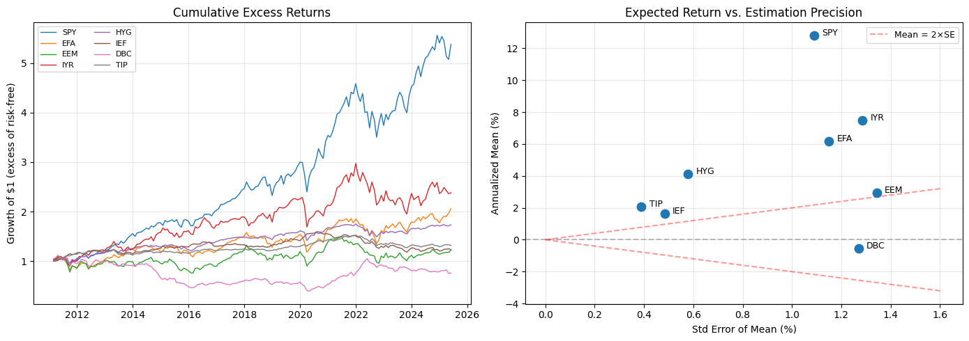
Expected returns are estimated from first moments—sample means. The standard error on an annualized mean is \(\sigma / \sqrt{T}\). For an asset with 15% annual volatility and 170 monthly observations, that’s \(15\% / \sqrt{170} \approx 1.15\%\)—about the same magnitude as the differences in expected returns across asset classes.
The optimizer doesn’t know this. It treats \(\hat{\mu}\) as truth and aggressively exploits any apparent return advantage, producing portfolios that are dominated by estimation noise.
From Shrinkage to Equilibrium#
One fix is to shrink the expected returns toward a common value, reducing the extreme differences that the optimizer exploits. But toward what? Shrinking toward the global mean (the average return across all assets) is a statistical convenience with no economic justification.
A better anchor comes from the CAPM. If the market portfolio is the tangency portfolio, then the expected returns that rationalize market-cap weights can be recovered by inverting the first-order condition:
where \(\delta\) is the risk aversion parameter and \(w_{mkt}\) is the vector of market-cap weights. These equilibrium returns are derived from \(\Sigma\) (well-estimated) rather than from sample means (noisy), so they produce stable portfolios by construction.
Adding Views#
Equilibrium returns are stable but generic—they reflect market consensus, not your beliefs. The Black-Litterman framework provides a disciplined way to tilt the portfolio toward investor views:
This is a Bayesian update: it blends a prior (equilibrium) with signals (views), where the tilt size depends on confidence. The result: controlled deviations from market-cap weights that reflect conviction without producing the extreme positions that plague naive MV.
Resources#
Course Materials#
Discussion 1.2: Optimizing Risk and Return — MV optimization, tangency portfolio, efficient frontier
Case Study C.1.2: MV Optimization of the Harvard Endowment — Tangency computation, TIPS sensitivity, regularized allocation
Case Study C.1.3: Constrained Optimization of the Harvard Endowment — Bounded optimization, Lagrange multipliers
Exercise E.1.2: Unconstrained Optimization — Tangency and GMV computation
Exercise E.1.3: Constrained Optimization — Position constraints
Discussion 4.1: CAPM — Equilibrium expected returns, market beta
Data#
File |
Description |
Frequency |
Date Range |
|---|---|---|---|
|
Prices, total returns, excess returns for 12 multi-asset ETFs |
Monthly |
2011–2025 |
The excess returns sheet provides returns in excess of the risk-free rate (SHV proxy), which is what enters the MV optimization directly. Use the 8-asset universe: SPY, EFA, EEM, IYR, HYG, IEF, DBC, TIP.
Data Preview#
import pandas as pd
import numpy as np
import matplotlib.pyplot as plt

DATA_PATH = '../../data/'

retsx = pd.read_excel(DATA_PATH + 'multi_asset_etf_data.xlsx',
                      sheet_name='excess returns', index_col=0, parse_dates=True)

UNIVERSE = ['SPY', 'EFA', 'EEM', 'IYR', 'HYG', 'IEF', 'DBC', 'TIP']
retsx = retsx[UNIVERSE].dropna()

print(f'Monthly excess returns: {retsx.shape[0]} months, {retsx.shape[1]} assets')
print(f'Date range: {retsx.index.min().date()} to {retsx.index.max().date()}')

# Summary statistics
stats = pd.DataFrame(index=UNIVERSE)
stats['Ann Mean (%)'] = retsx.mean() * 12 * 100
stats['Ann Vol (%)'] = retsx.std() * np.sqrt(12) * 100
stats['Sharpe'] = (retsx.mean() / retsx.std()) * np.sqrt(12)
stats['SE of Mean (%)'] = (retsx.std() / np.sqrt(len(retsx))) * np.sqrt(12) * 100

print('\nAnnualized statistics (monthly excess returns):')
stats.round(2)
Monthly excess returns: 172 months, 8 assets
Date range: 2011-02-28 to 2025-05-31

Annualized statistics (monthly excess returns):
| Ann Mean (%) | Ann Vol (%) | Sharpe | SE of Mean (%) | |
|---|---|---|---|---|
| SPY | 12.81 | 14.28 | 0.90 | 1.09 |
| EFA | 6.18 | 15.09 | 0.41 | 1.15 |
| EEM | 2.93 | 17.62 | 0.17 | 1.34 |
| IYR | 7.49 | 16.87 | 0.44 | 1.29 |
| HYG | 4.14 | 7.59 | 0.54 | 0.58 |
| IEF | 1.64 | 6.34 | 0.26 | 0.48 |
| DBC | -0.53 | 16.66 | -0.03 | 1.27 |
| TIP | 2.05 | 5.11 | 0.40 | 0.39 |
fig, axes = plt.subplots(1, 2, figsize=(14, 5))

# Cumulative returns
ax = axes[0]
for col in UNIVERSE:
    cum = (1 + retsx[col]).cumprod()
    ax.plot(cum.index, cum, linewidth=1, label=col)
ax.set_ylabel('Growth of $1 (excess of risk-free)')
ax.set_title('Cumulative Excess Returns')
ax.legend(fontsize=8, ncol=2)
ax.grid(True, alpha=0.3)

# Mean vs SE scatter
ax = axes[1]
ax.scatter(stats['SE of Mean (%)'], stats['Ann Mean (%)'], s=80, zorder=5)
for ticker in UNIVERSE:
    ax.annotate(ticker, (stats.loc[ticker, 'SE of Mean (%)'],
                        stats.loc[ticker, 'Ann Mean (%)']),
               textcoords='offset points', xytext=(8, 0), fontsize=9)
ax.axhline(0, color='gray', ls='--', alpha=0.5)
# Add 45-degree 'significance' line: mean = 2 * SE
se_range = np.linspace(0, stats['SE of Mean (%)'].max() * 1.2, 50)
ax.plot(se_range, 2 * se_range, 'r--', alpha=0.4, label='Mean = 2×SE')
ax.plot(se_range, -2 * se_range, 'r--', alpha=0.4)
ax.set_xlabel('Std Error of Mean (%)')
ax.set_ylabel('Annualized Mean (%)')
ax.set_title('Expected Return vs. Estimation Precision')
ax.legend(fontsize=9)
ax.grid(True, alpha=0.3)

plt.tight_layout()
plt.show()
Questions#
Q1: Diagnosing Estimation Error (Updated)#
In the Harvard case, you saw that adjusting the TIPS mean by less than one standard error changed the tangency portfolio dramatically. That was a single perturbation. Here you will quantify the problem systematically.
Using the 8-asset universe:
Estimate expected returns and the covariance matrix from the full sample. Compute the tangency portfolio weights.
Generate 500 bootstrap resamples (sample with replacement from the monthly returns). For each resample, re-estimate the mean vector and covariance matrix and recompute the tangency portfolio.
Plot the distribution of each asset’s weight across the 500 bootstraps (e.g., box plots or violin plots). Report the mean weight and bootstrap standard error of each weight.
For each asset, compute a 95% confidence interval for the tangency weight using the bootstrap percentile method (2.5th and 97.5th percentiles of the bootstrap distribution). Present the results in a table. What do these intervals tell you about how precisely the optimizer can identify the “optimal” weight?
Repeat the bootstrap analysis for the GMV portfolio (which ignores expected returns entirely). Report 95% confidence intervals for the GMV weights. How does GMV weight precision compare to tangency?
What does this tell you about which input—expected returns or covariances—is the source of instability?
Q2: Simple Methods vs. the Optimizer#
Set up a rolling out-of-sample backtest: estimate on a trailing 60-month (5-year) window, hold the resulting portfolio for 1 month, then roll forward.
Compare four allocation methods:
Naive MV (tangency): unconstrained, using sample mean and covariance from the estimation window
Equal weight (1/N): no estimation at all
Global minimum variance (GMV): uses only the covariance matrix, ignores expected returns
Long-only constrained MV: maximize Sharpe ratio with weights constrained to \([0, 1]\)
For each method, report: out-of-sample annualized mean return, volatility, Sharpe ratio, maximum drawdown, and average monthly turnover (defined as \(\frac{1}{2}\sum_i |w_{i,t} - w_{i,t-1}|\), where the weights before rebalancing reflect one month of return drift).
Also plot the weight evolution over time for each method. Which methods produce stable allocations? Which are erratic?
Q2 Part B (New): Binding Constraints and the Optimizer#
This extends Q2’s constrained MV method (method 4). In that method, you imposed long-only bounds \(w_i \in [0, 1]\). Here, use cvxpy to solve the constrained problem and examine which constraints the optimizer is fighting against.
Formulate the constrained tangency portfolio as a cvxpy problem. In addition to the long-only constraint, add a position-size cap: no single asset can exceed 25% of the portfolio. Since the Sharpe ratio is not directly convex, use the standard reformulation: fix the return level and minimize variance, then rescale.
The constraint \(w_i \leq 0.25 \cdot \mathbf{1}'w\) enforces that each weight is at most 25% of the total. After solving, rescale so that \(\mathbf{1}'w = 1\).
import cvxpy as cp

n = len(mu)
w = cp.Variable(n)
objective = cp.Minimize(cp.quad_form(w, Sigma))
ub_constraint = w <= 0.25 * cp.sum(w)
constraints = [mu @ w == 1, w >= 0, ub_constraint]
prob = cp.Problem(objective, constraints)
prob.solve()
w_opt = w.value / w.value.sum()       # rescale to budget constraint
duals = ub_constraint.dual_value       # shadow prices on the position cap
In your rolling backtest, for each estimation window:
Solve the constrained problem and record the dual variables (shadow prices) associated with the position-size constraints.
A binding constraint is one where the dual variable is nonzero — the optimizer wants to exceed the bound.
Report: which assets hit the 25% cap most frequently across the rolling windows? Does the set of binding constraints change over time — for example, during the high-correlation regime of 2020? Relate binding frequency to properties of the covariance matrix in each estimation window.
Q3: Shrinking Toward Stability#
Q1 showed that tangency weights are wildly unstable while GMV weights are not. This suggests expected returns are the problem—but how do we know the covariance matrix isn’t also contributing? Before fixing expected returns, test the covariance directly.
a) Covariance shrinkage (Ledoit-Wolf) (Updated)
The sample covariance matrix \(\hat{\Sigma}\) is an unbiased estimator, but with 8 assets and 172 months it can still amplify estimation noise—particularly in the off-diagonal terms that drive the optimizer’s hedging trades. Ledoit-Wolf shrinkage addresses this by pulling the sample covariance toward a structured target:
where \(F\) is a low-dimensional target (typically the constant-correlation or single-factor covariance matrix) and \(\delta \in [0, 1]\) is chosen to minimize expected estimation loss. The idea is the same as mean shrinkage: trade a small amount of bias for a large reduction in variance. Use sklearn.covariance.LedoitWolf to estimate \(\hat{\Sigma}_{LW}\).
Recompute the tangency portfolio using the Ledoit-Wolf covariance (keeping sample means unchanged). Then repeat the bootstrap from Q1: in each resample, apply Ledoit-Wolf to the bootstrap covariance and recompute the tangency. Does covariance shrinkage meaningfully reduce weight instability? Compare the bootstrap standard deviations to those from Q1.
Aside: The simplest form of covariance regularization is adding a small multiple of the identity to the diagonal: \(\hat{\Sigma}_{reg} = \hat{\Sigma} + \lambda I\). This improves the condition number directly—exactly the diagonal-loading intuition from class. It is also equivalent to ridge regression when the tangency portfolio is viewed as a regression problem (\(w \propto \Sigma^{-1}\mu\) corresponds to an OLS coefficient). Ledoit-Wolf is a more sophisticated version of this same idea, choosing the shrinkage target and intensity optimally. Note that weights from \((\hat{\Sigma} + \lambda I)^{-1}\mu\) do not automatically sum to one and must be rescaled to satisfy the budget constraint.
b) Mean shrinkage (Updated)
Now turn to the expected returns. Shrink toward the global mean:
where \(\bar{\mu}\) is the cross-sectional average of all sample means and \(\alpha \in [0, 1]\) controls shrinkage intensity.
For \(\alpha \in \{0, 0.25, 0.50, 0.75, 1.0\}\), compute the tangency portfolio weights. How do the weights change as \(\alpha\) increases? What happens at \(\alpha = 1\)?
Now choose an \(\alpha\) for the bootstrap analysis. Repeat the Q1 bootstrap at your chosen \(\alpha\): does mean shrinkage reduce weight variability more than covariance shrinkage did in part (a)? Is there an \(\alpha\) that minimizes bootstrap weight variance? Is that the \(\alpha\) you would actually recommend to a portfolio manager — or are there reasons to prefer a different value?
c) Out-of-sample test
Add the shrinkage tangency at your chosen \(\alpha\) to the rolling OOS backtest from Q2. Does it improve out-of-sample performance? If you tried multiple values of \(\alpha\) in part (b), does the \(\alpha\) that looks best in-sample (lowest weight variance) also perform best out of sample?
d) The shrinkage target
Comment on the choice of target. Shrinking expected returns toward the global mean is a statistical convenience—it says every asset has the same expected return, regardless of risk. Why might this be a poor anchor? What would be an economically motivated alternative?
Q4: Equilibrium Returns#
Instead of shrinking toward an arbitrary target, derive expected returns from an economic model. If the market portfolio is the tangency portfolio (as CAPM implies), then the expected returns that rationalize market-cap weights are:
where \(\delta\) is the risk aversion parameter and \(w_{mkt}\) is the vector of market-cap weights. Calibrate \(\delta\) using the market Sharpe ratio: \(\delta = SR_{mkt} / \sigma_{mkt}\). Use SPY as the market proxy and estimate the Sharpe ratio and volatility from the same sample window as your \(\Sigma\) estimate.
Use the approximate market-cap weights below:
Asset |
SPY |
EFA |
EEM |
IYR |
HYG |
IEF |
DBC |
TIP |
|---|---|---|---|---|---|---|---|---|
Weight |
35% |
20% |
10% |
5% |
5% |
15% |
3% |
7% |
a) Compute the equilibrium returns \(\pi\). Compare them to the sample means from Q1. Where do they agree? Where do they disagree most?
b) Use \(\pi\) as the expected return input and compute the tangency portfolio. What weights do you get?
c) Repeat the bootstrap analysis using equilibrium returns (re-estimate \(\Sigma\) in each bootstrap but use \(\pi = \delta \hat{\Sigma}_{boot} w_{mkt}\) each time). How stable are the weights compared to Q1?
d) Test whether \(\delta\) matters: compute the tangency portfolio using \(\delta = 2.0\) and \(\delta = 4.0\). Do the weights change? Explain why or why not.
e) Add the equilibrium-based portfolio to the OOS backtest from Q2. Report the same performance metrics.
Q5: Incorporating Views#
Equilibrium returns are stable but generic. An allocator who believes US equities will continue to outperform needs a way to tilt the portfolio without destroying the stability.
Consider two investor views:
View 1 (relative): US equities (SPY) will outperform developed international (EFA) by 3% per year over the next 5 years.
View 2 (absolute): Commodities (DBC) will return 2% per year (below the equilibrium return, reflecting skepticism about commodity performance).
a) Express each view as a linear restriction using a pick matrix \(P\) and a view vector \(v\). For View 1: a row of \(P\) with +1 on SPY and −1 on EFA.
b) Blend the views with the equilibrium prior using the Black-Litterman formula:
Use \(\tau = 0.05\). For the view uncertainty matrix, start with \(\Omega = \text{diag}(P \cdot \tau\Sigma \cdot P')\).
c) Compute optimal weights using \(\hat{\mu}_{BL}\). How do they differ from equilibrium weights? From sample-mean tangency weights?
d) Sensitivity analysis: Scale \(\Omega_{11}\) (the uncertainty on View 1) from very confident (multiply by 0.1) to very uncertain (multiply by 10). Plot the weight on SPY and EFA as a function of view confidence. What happens at the extremes?
Compare this to the Harvard TIPS exercise: there, changing the expected return by less than one standard error caused a 75-percentage-point weight swing. How does the BL framework handle the same type of perturbation?
e) (Updated) Your own view: Propose a third view grounded in current market conditions. It can be absolute or relative, and it should involve at least one asset not already covered by Views 1–2. Express it as a row of \(P\) and an entry in \(v\), choose a confidence level for \(\Omega\), and add it to the BL model alongside the first two views. Show how the resulting weights change relative to the two-view allocation from part (c). Justify both the view itself and your choice of confidence.
Q6: Synthesis#
Create a summary table of out-of-sample performance across all methods tested:
Method |
OOS Sharpe |
OOS Vol |
Max Drawdown |
Turnover |
|---|---|---|---|---|
Naive MV (tangency) |
— |
— |
— |
— |
Equal Weight (1/N) |
— |
— |
— |
— |
GMV |
— |
— |
— |
— |
Constrained MV |
— |
— |
— |
— |
Shrinkage MV (your α) |
— |
— |
— |
— |
Equilibrium MV |
— |
— |
— |
— |
BL (2 views) |
— |
— |
— |
— |
Based on your analysis:
Which approach would you recommend for a long-horizon institutional investor? What tradeoffs does your recommendation involve? State the specific conditions under which you would switch to a different method.
When does it make sense to deviate from market-cap weights? How confident must an allocator be in a view to justify a meaningful tilt?
Consider the current market environment, where US large-cap equities (especially mega-cap tech) have dramatically outperformed international markets. How would the BL framework handle an allocator’s view on whether this outperformance will persist?