TA Review - Dynamics#
TA: Tobias del Pozo
Lecture 3, Autumn 2026. VaR, risk measures, and time diversification.
Thank you to Younghun Lee for materials from previous years.
The figures and tables use the review’s historical samples. Rerunning with updated course data can change the estimates. The stock exercise uses the frozen 2015–2025 weekly sample.
import pandas as pd
import numpy as np
import matplotlib.pyplot as plt
import scipy.stats as stats
import statsmodels.api as sm

plt.style.use("dark_background")
pd.set_option("display.max_columns", None)
pd.set_option("display.max_rows", None)

df = pd.read_excel(
    "../data/risk_etf_data.xlsx", sheet_name="total returns", index_col=0, parse_dates=True
)
df[["SPY", "VEA", "GLD"]].head().style.format({c: "{:.2%}" for c in df}, na_rep="n/a").format_index("{:%Y-%m-%d}")
| SPY | VEA | GLD | |
|---|---|---|---|
| Date | |||
| 2017-01-04 | 0.59% | 1.22% | 0.35% |
| 2017-01-05 | -0.08% | 0.89% | 1.55% |
| 2017-01-06 | 0.36% | -0.40% | -0.74% |
| 2017-01-09 | -0.33% | -0.24% | 0.82% |
| 2017-01-10 | 0.00% | 0.11% | 0.43% |
Definition#
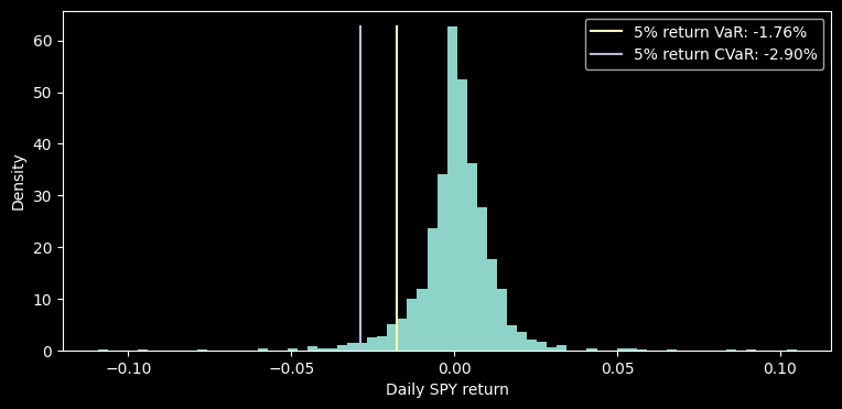
The Value-at-Risk (VaR) is simply a quantile of the distribution.
In this class, we just use the quantile of the returns distribution. So: VaR(0.05) is the 5% quantile of the returns distribution.
Conditional Value at Risk (CVaR)
For continuous return distributions, Conditional Value at Risk (CVaR) is a measure of the expected loss given that the loss is greater than the VaR. It is a measure of the expected downside risk. In this class, we just use the mean of the returns that are less than the VaR. So: CVaR(0.05) is the mean of the returns that are less than the 5% quantile of the returns distribution.
With discrete outcomes or ties, expected shortfall averages the worst \(q\) probability mass, including only the needed fraction at the cutoff.
Non-Parametric VaR#
The easiest way to calculate VaR is “non-parametric VaR”, this just looks at historical returns and finds the percentile of returns that correspond to the confidence level you want.
np.random.seed(7)
spy_daily = df["SPY"].dropna()
q = 0.05
empirical_var = spy_daily.quantile(q)
empirical_es = spy_daily[spy_daily <= empirical_var].mean()

fig, ax = plt.subplots(figsize=(9, 4))
density, _, _ = ax.hist(spy_daily, bins=70, density=True, alpha=1)
for value, label in [
    (empirical_var, "5% return VaR"),
    (empirical_es, "5% return CVaR"),
]:
    ax.plot([value, value], [0, density.max()], label=f"{label}: {value:.2%}")
ax.set(xlabel="Daily SPY return", ylabel="Density")
ax.legend()
plt.show()
Parametric VaR#
To get around this, we typically use some kind of parametric VaR, where we try to enforce some distribution/model on the returns and then use that to calculate VaR. The simplest way to do this is to assume returns are normally distributed, and therefore:
Where \(\Phi^{-1}\) is the inverse CDF of the standard normal distribution. So if we wanted to get 5% VaR, we would get:
And again, we could calculate this non-parametrically, or if we use the normal distribution, we can get a closed form solution:
mu_daily, sigma_daily = spy_daily.mean(), spy_daily.std()
tail_comparison = pd.DataFrame(
    {
        "Empirical": [empirical_var, empirical_es],
        "Normal model": [
            mu_daily + sigma_daily * stats.norm.ppf(q),
            mu_daily - sigma_daily * stats.norm.pdf(stats.norm.ppf(q)) / q,
        ],
    },
    index=["5% return VaR", "5% return CVaR"],
)
tail_comparison.style.format({c: "{:.2%}" for c in tail_comparison}, na_rep="n/a")
| Empirical | Normal model | |
|---|---|---|
| 5% return VaR | -1.76% | -1.89% |
| 5% return CVaR | -2.90% | -2.39% |
Coherent Risk Measures#
Risk Measures#
Do all these metrics have the properties which will make for a useful risk measure?
Define the following notation:
two risky payoffs (in USD) \(\Pi_j, \Pi_k\).
\(\alpha\): amount of cash holding.
A risk measure \(\varrho\) measures
a dollar amount of losses–not the expected losses, but rather the amount of losses that could result
equivalently, the amount of capital required to protect against losses
Different risk measures will give different answers to this question.
volatility (std.dev.)
variance
quantile
If a risk measure of a risky position, \(\varrho(\Pi_j)\) is negative, it indicates an amount of capital that could be withdrawn.
Coherence#
For a risk measure to be sensible for measuring risk capital, it should have certain features.
A coherent risk, \(\varrho\), measure satisfies the following properties:
Translation Invariance#
Adding cash to a position reduces the capital needed to support it one-for-one.
A stock plus cash needs less additional capital support (protection) than the stock alone.
If this were not true, it would say that, for risk purposes, combining the cash with the risky assets is different than holding the cash in a separate account.
Positive Homogeneity#
For any positive scaling, \(\lambda>0\),
The risk capital scales linearly with the position.
Monotonicity#
If \(\Pi_j\geq\Pi_k\) in every state (almost surely) then the risk measure of \(\Pi_j\) is no greater:
For instance, suppose that
\(\Pi_k\) is a stock
\(\Pi_j\) is the same stock plus a long put option
Then this definition requires that a coherent risk measure would assign no greater risk to \(\Pi_j\).
Subadditive#
The risk of the total is less than the sum of its parts:
This condition states that there is a diversification benefit, or at least, no harm.
Margin requirement#
If this condition did not hold, it would say that there is a direct benefit to splitting assets across accounts, rather than having them net for the margin requirement.
Is \(\text{VaR}\) a coherent risk measure?
No. In general, it is not subadditive.
Is \(\sigma^2\) a coherent risk measure?
No. It’s not subadditive. Eg. \(X\) and \(Y\) are positively correlated at with correlation 1, then \(\sigma^2(X+Y) = \sigma^2(X) + \sigma^2(Y) + 2\sigma(X)\sigma(Y) > \sigma^2(X) + \sigma^2(Y)\).
\(\sigma^2\) also doesn’t have homogeneity, since \(\sigma^2(\lambda X) = \lambda^2\sigma^2(X)\).
Is \(\sigma\) a coherent risk measure?
No. Standard deviation is subadditive and positively homogeneous, but it fails translation invariance and monotonicity. Adding cash leaves standard deviation unchanged, although it reduces the required risk capital.
losses = pd.DataFrame(0.0, index=range(100), columns=["A", "B"])
losses.loc[0:3, "A"] = 100
losses.loc[4:7, "B"] = 100
losses["A + B"] = losses["A"] + losses["B"]

loss_risk = pd.DataFrame(
    {
        "Loss VaR (95%)": np.quantile(losses, 0.95, axis=0, method="inverted_cdf"),
        "Loss CVaR (95%)": np.sort(losses.to_numpy(), axis=0)[-5:].mean(axis=0),
    },
    index=losses.columns,
)
display(losses.value_counts().rename("States out of 100").reset_index().style.format({"A": "${:.0f}", "B": "${:.0f}", "A + B": "${:.0f}", "States out of 100": "{:.0f}"}, na_rep="n/a").hide(axis="index"))
loss_risk.style.format({c: "${:.0f}" for c in loss_risk}, na_rep="n/a")
| A | B | A + B | States out of 100 |
|---|---|---|---|
| $0 | $0 | $0 | 92 |
| $0 | $100 | $100 | 4 |
| $100 | $0 | $100 | 4 |
| Loss VaR (95%) | Loss CVaR (95%) | |
|---|---|---|
| A | $0 | $80 |
| B | $0 | $80 |
| A + B | $100 | $100 |
Normal VaR#
Is Normal VaR coherent?
For jointly normal payoffs and a loss confidence level above 50%, VaR is subadditive. Normal marginal distributions alone do not establish this result.
CVaR#
Is CVaR coherent?
For a normal distribution?
For the examples above?
Also yes. In general CVaR is coherent. And from above, \(\mathrm{CVaR}(A+B)=100 \le 80+80=160\).
Conditional Moments#
Whether using a normal model or something else, we want to allow \(\text{VaR}\) to be dynamic across time. That is, we want the conditional \(\text{VaR}\), utilizing info up to time \(t\) (which we’re obviously doing implicitly before, but we maybe want to be more dynamic about it).
For normal \(\text{VaR}\) this means having a dynamic model of the volatility.
You can typically ignore the mean.
Why can we ignore the mean? Well, typically you have a separate model for the mean (it can be useful to model the mean and volatility separately). So you can think of \(r\) here are the residuals/returns after demeaning, not the raw returns.
Below, we use the notation that \(\sigma_t^2\) is estimated using data through \(t-1\) as an estimate of what variance will be the next period (\(t\)).
Expanding#
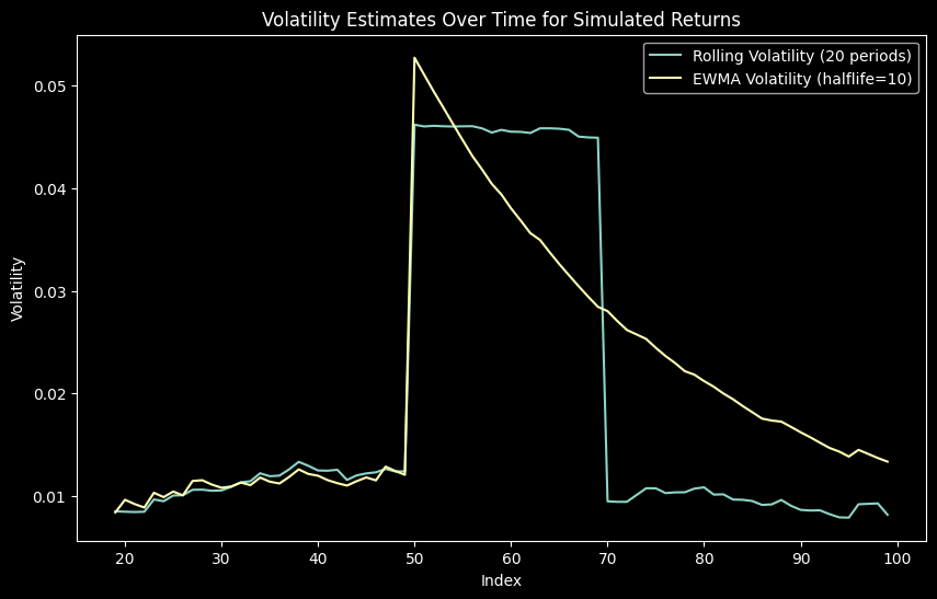
Rolling#
What is one issue with the rolling method?
Well, if we have one period of very high volatility, and then we’re back to low volatility, our rolling window will have a gap up, and then a gap down, which makes it very weird.
What is one issue with the expanding method?
Well, similarly, the market can change!
EWMA#
The exponential weighted moving average (EWMA) puts more weight on more recent data by setting a geometric decay parameter, \(\lambda\in [0, 1]\). (Typically \(\lambda\) will be in \((.9,1)\).
This is often written in the form,
Or, we can specify the half-life, which is the amount of time it takes for the weight to decay by half. Then, we can calculate \(\lambda\) as:
rv = np.random.normal(loc=0, scale=0.01, size=100)

rv[50] = -0.2

rv_series = pd.Series(rv)
rv_volatility = rv_series.rolling(window=20).std()
rv_vol_ewm = rv_series.ewm(halflife=10, min_periods=20).std()

fig, ax = plt.subplots(figsize=(10, 6))
ax.plot(rv_volatility, label="Rolling Volatility (20 periods)")
ax.plot(rv_vol_ewm, label="EWMA Volatility (halflife=10)")
ax.set_title("Volatility Estimates Over Time for Simulated Returns")
ax.set_xlabel("Index")
ax.set_ylabel("Volatility")
ax.legend()
plt.show()
Evaluating VaR#
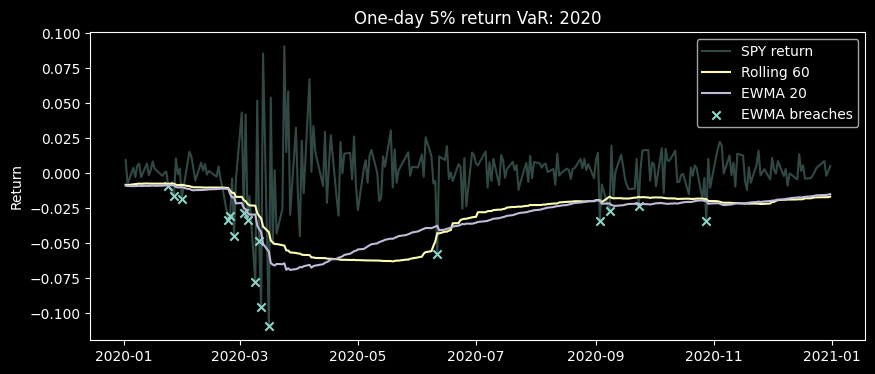
The Hit Test is a common way of backtesting a VaR methodology.
It checks historically what the daily VaR would have been, given the information known at that time. It compares this to the actual performance for the day.
If the VaR is working well, then the day-t loss should only exceed the day-\(t\) \(\Gamma^{\text{VaR}_{q,1}}\) with a probability of \(q.\)
But what if future market environment is very different than past environment with which fit test was run? Many VaR models looked okay before the 2007-2008 crisis hit!
rolling_variance = spy_daily.pow(2).rolling(60).mean()
ewma_variance = spy_daily.pow(2).ewm(halflife=20, adjust=False, min_periods=60).mean()

# Forecast day t with information available through day t-1.
var_forecasts = pd.DataFrame(
    {
        "Rolling 60": stats.norm.ppf(q) * np.sqrt(rolling_variance.shift(1)),
        "EWMA 20": stats.norm.ppf(q) * np.sqrt(ewma_variance.shift(1)),
    }
)
evaluation = spy_daily.rename("Return").to_frame().join(var_forecasts).dropna()
breaches = evaluation[var_forecasts.columns].gt(evaluation["Return"], axis=0)
coverage = pd.DataFrame(
    {
        "Observations": len(evaluation),
        "Breaches": breaches.sum(),
        "Hit rate": breaches.mean(),
        "Target": q,
    }
)
display(coverage.style.format({"Observations": "{:.0f}", "Breaches": "{:.0f}", "Hit rate": "{:.2%}", "Target": "{:.2%}"}, na_rep="n/a"))

window = evaluation.loc["2020"]
fig, ax = plt.subplots(figsize=(10, 4))
ax.plot(window.index, window["Return"], alpha=0.35, label="SPY return")
for method in var_forecasts:
    ax.plot(window.index, window[method], label=method)
breached = window.index[breaches.loc[window.index, "EWMA 20"]]
ax.scatter(breached, window.loc[breached, "Return"], marker="x", label="EWMA breaches")
ax.set(title="One-day 5% return VaR: 2020", ylabel="Return")
ax.legend()
plt.show()
| Observations | Breaches | Hit rate | Target | |
|---|---|---|---|---|
| Rolling 60 | 2072 | 126 | 6.08% | 5.00% |
| EWMA 20 | 2072 | 123 | 5.94% | 5.00% |
VaR Hit Rates#
We can evaluate our VaR model by looking at the hit rate.
Our parametric VaR will typically only be as good as our forward looking volatility estimates.
Barnstable and Long-Run Risk#
HBS Case#
The Risk of Stocks in the Long-Run: The Barnstable College Endowment#
1 Barnstable’s Philosophy#
What has Barnstable’s investment strategy been in the past?
Explain the logic behind their view that stocks are safer in the long run.
What assumptions underlie Barnstable’s belief in the long-run safety of stocks?
Barnstable’s estimates of mean and volatility are based on the subsample of 1965 to 1999.
Notation#
\(r\) = level return rates
\(R\) = cumulative return factor
\(\texttt{r}\) = log return rates
Cumulative Return Risk and Autocorrelation#
Log cumulative returns are simply a portfolio of single-period returns.
Define \(\mu\) and \(\sigma^2\) as
For the \(h\)-period log return,
The idea here is that the covariances determine the overall risk, but we are assuming that the returns are i.i.d., so the covariances are zero, and therefore the variance of the \(h\)-period log return is simply \(h\sigma^2\). Under the additional assumption that log excess returns are normally distributed, the probability of underperforming a threshold \(r^*\) over a time period \(T\) directly comes from a z-score.
Sol)#
Let annualized mean and volatility of log excess return as \(\mu\) and \(\sigma\), then we can see
As such,
barnstable = pd.read_excel(
    "../data/barnstable_analysis_data.xlsx",
    sheet_name="data",
    index_col=0,
    parse_dates=True,
)[["SPX", "TB1M"]].dropna()
# Relative log wealth is log(1 + market return) minus log(1 + bill return).
log_excess = np.log1p(barnstable["SPX"]) - np.log1p(barnstable["TB1M"])
calibrations = {}
for start_year, end_year in [("1965", "1999"), ("2000", "2024"), ("1965", "2024")]:
    sample = log_excess.loc[start_year:end_year]
    mu_log = sample.mean() * 12
    sigma_log = sample.std() * np.sqrt(12)
    calibrations[f"{start_year}–{end_year}"] = {
        "Months": len(sample),
        "Annual log premium": mu_log,
        "Annual log volatility": sigma_log,
        "P(underperform, 15 years)": stats.norm.cdf(-np.sqrt(15) * mu_log / sigma_log),
        "P(underperform, 30 years)": stats.norm.cdf(-np.sqrt(30) * mu_log / sigma_log),
    }
barnstable_stats = pd.DataFrame(calibrations).T
display(
    barnstable_stats.style.format(
        {
            "Months": "{:.0f}",
            **{col: "{:.2%}" for col in barnstable_stats if col != "Months"},
        }, na_rep="n/a"
    )
)
| Months | Annual log premium | Annual log volatility | P(underperform, 15 years) | P(underperform, 30 years) | |
|---|---|---|---|---|---|
| 1965–1999 | 419 | 5.71% | 15.04% | 7.08% | 1.88% |
| 2000–2024 | 300 | 5.81% | 15.40% | 7.19% | 1.94% |
| 1965–2024 | 719 | 5.75% | 15.18% | 7.12% | 1.90% |
Time Diversification#
Under the i.i.d. model with finite variance, the variance of the average annual log return approaches zero as the investment horizon grows.
This statement concerns the average log return, conditional on the assumed model and parameters.
However, the variance of the cumulative return, \(r^{\log}_{t,t+h}\) is still growing.
So-called time diversification depends on the risk one is measuring.
mu_log = barnstable_stats.loc["1965–1999", "Annual log premium"]
sigma_log = barnstable_stats.loc["1965–1999", "Annual log volatility"]
h = np.array([1, 5, 15, 30])
horizon_risk = pd.DataFrame(
    {
        "P(underperform)": stats.norm.cdf(-np.sqrt(h) * mu_log / sigma_log),
        "Cumulative log-return std.": sigma_log * np.sqrt(h),
        "Annualized log-return std.": sigma_log / np.sqrt(h),
    },
    index=pd.Index(h, name="Years"),
)
horizon_risk.style.format({c: "{:.2%}" for c in horizon_risk}, na_rep="n/a")
| P(underperform) | Cumulative log-return std. | Annualized log-return std. | |
|---|---|---|---|
| Years | |||
| 1 | 35.22% | 15.04% | 15.04% |
| 5 | 19.81% | 33.63% | 6.73% |
| 15 | 7.08% | 58.25% | 3.88% |
| 30 | 1.88% | 82.38% | 2.75% |
base = barnstable_stats.loc["1965–1999"]
# IID standard error of the annualized mean; volatility is held fixed.
mean_se = base["Annual log volatility"] * np.sqrt(12 / base["Months"])
horizons = np.arange(1, 31)
mean_sensitivity = {}
fig, ax = plt.subplots(figsize=(9, 4))
for shift, label in [
    (-1, "Mean − 1 standard error"),
    (0, "Estimated mean"),
    (1, "Mean + 1 standard error"),
]:
    assumed_mean = base["Annual log premium"] + shift * mean_se
    probability = stats.norm.cdf(
        -np.sqrt(horizons) * assumed_mean / base["Annual log volatility"]
    )
    ax.plot(horizons, probability, label=label)
    mean_sensitivity[label] = {
        "Annual log premium": assumed_mean,
        "P(underperform, 30 years)": probability[-1],
    }
ax.set(
    title="Barnstable: sensitivity to the estimated mean",
    xlabel="Horizon (years)",
    ylabel="Model-implied underperformance probability",
)
ax.legend()
plt.show()
pd.DataFrame(mean_sensitivity).T.style.format({c: "{:.2%}" for c in next(iter(mean_sensitivity.values()))}, na_rep="n/a")
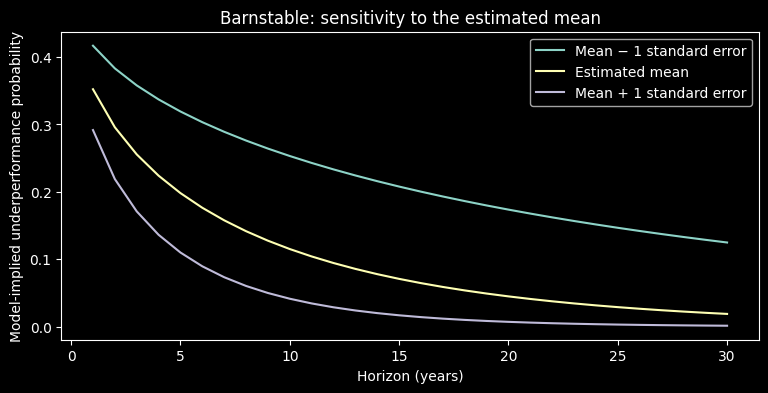
| Annual log premium | P(underperform, 30 years) | |
|---|---|---|
| Mean − 1 standard error | 3.16% | 12.48% |
| Estimated mean | 5.71% | 1.88% |
| Mean + 1 standard error | 8.25% | 0.13% |
Stock Portfolio Exercise#
spx = pd.read_excel(
    "../data/spx_returns_weekly_legacy_2025.xlsx", sheet_name="s&p500 rets", index_col=0, parse_dates=True
)[["AAPL", "META", "NVDA", "TSLA"]]
spx.head().style.format({c: "{:.2%}" for c in spx}, na_rep="n/a").format_index("{:%Y-%m-%d}")
| AAPL | META | NVDA | TSLA | |
|---|---|---|---|---|
| Date | ||||
| 2015-01-09 | 2.45% | -0.91% | -0.93% | -5.77% |
| 2015-01-16 | -5.37% | -3.29% | 0.08% | -6.58% |
| 2015-01-23 | 6.59% | 3.53% | 3.76% | 4.26% |
| 2015-01-30 | 3.70% | -2.47% | -7.26% | 1.15% |
| 2015-02-06 | 1.91% | -1.90% | 6.23% | 6.76% |
1.1 Full Sample Vol/VaR/CVaR#
stds = spx.std() * np.sqrt(52)
var = spx.quantile(0.05)
cvar = spx[spx <= var].mean()
summary_risk = pd.DataFrame(
    {"Annualized Volatility": stds, "VaR(0.05)": var, "CVaR(0.05)": cvar}
)
summary_risk.style.format({c: "{:.2%}" for c in summary_risk}, na_rep="n/a")
| Annualized Volatility | VaR(0.05) | CVaR(0.05) | |
|---|---|---|---|
| AAPL | 27.66% | -5.64% | -8.31% |
| META | 35.13% | -7.00% | -10.32% |
| NVDA | 46.33% | -8.69% | -11.65% |
| TSLA | 58.64% | -11.74% | -14.78% |
1.2 Equally Weighted Portfolio#
weights = np.array([0.25, 0.25, 0.25, 0.25])
portfolio_rets = spx.dot(weights)

std_port = portfolio_rets.std() * np.sqrt(52)
var_port = portfolio_rets.quantile(0.05)
cvar_port = portfolio_rets[portfolio_rets <= var_port].mean()
pd.DataFrame(
    {
        "Annualized Volatility": [std_port],
        "VaR(0.05)": [var_port],
        "CVaR(0.05)": [cvar_port],
    },
    index=["Equally Weighted Portfolio"],
) .style.format({"Annualized Volatility": "{:.2%}", "VaR(0.05)": "{:.2%}", "CVaR(0.05)": "{:.2%}"}, na_rep="n/a")
| Annualized Volatility | VaR(0.05) | CVaR(0.05) | |
|---|---|---|---|
| Equally Weighted Portfolio | 31.55% | -6.19% | -8.50% |
1.3 Replacing TSLA with Cash#
Keep 25% in each of the other three stocks and hold 25% in cash, assumed to earn zero over the measurement period.
weights = np.array([0.25, 0.25, 0.25, 0.0])

portfolio_rets_no_tsla = spx.dot(weights)
std_port = portfolio_rets_no_tsla.std() * np.sqrt(52)
var_port = portfolio_rets_no_tsla.quantile(0.05)
cvar_port = portfolio_rets_no_tsla[portfolio_rets_no_tsla <= var_port].mean()
pd.DataFrame(
    {
        "Annualized Volatility": [std_port],
        "VaR(0.05)": [var_port],
        "CVaR(0.05)": [cvar_port],
    },
    index=["25% Cash"],
) .style.format({"Annualized Volatility": "{:.2%}", "VaR(0.05)": "{:.2%}", "CVaR(0.05)": "{:.2%}"}, na_rep="n/a")
| Annualized Volatility | VaR(0.05) | CVaR(0.05) | |
|---|---|---|---|
| 25% Cash | 21.84% | -4.25% | -6.05% |
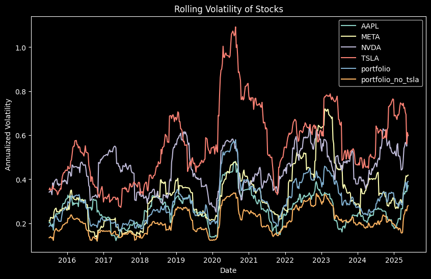
2.1 Volatility#
fig, ax = plt.subplots(figsize=(10, 6))
spx["Equally Weighted"] = portfolio_rets
spx["25% Cash"] = portfolio_rets_no_tsla

rolling_vol = spx.rolling(window=26, min_periods=26).std() * np.sqrt(52)

ax.plot(rolling_vol, label=rolling_vol.columns)
ax.set_title("Rolling Volatility of Stocks")
ax.set_xlabel("Date")
ax.set_ylabel("Annualized Volatility")
ax.legend()
plt.show()
Assume Mean is 0, and Calculate VaR/CVaR#
last_rolling_vol = rolling_vol.iloc[-1]

var_95 = stats.norm.ppf(0.05) * last_rolling_vol / np.sqrt(52)
cvar_95 = (
    -(last_rolling_vol / np.sqrt(52)) * stats.norm.pdf(stats.norm.ppf(0.05)) / 0.05
)

print("Conditional (using last rolling volatility)")
display(
    pd.DataFrame(
        {
            "Annualized Volatility": last_rolling_vol,
            "VaR(0.05) assuming normality": var_95,
            "CVaR(0.05) assuming normality": cvar_95,
        }
    ).style.format({"Annualized Volatility": "{:.2%}", "VaR(0.05) assuming normality": "{:.2%}", "CVaR(0.05) assuming normality": "{:.2%}", "VaR(0.05)": "{:.2%}", "CVaR(0.05)": "{:.2%}"}, na_rep="n/a")
)
print("Unconditional (empirical CDF)")
display(
    pd.DataFrame(
        {
            "Annualized Volatility": (full_std := spx.std() * np.sqrt(52)),
            "VaR(0.05)": (var_tmp := spx.quantile(0.05)),
            "CVaR(0.05)": spx[spx <= var_tmp].mean(),
        }
    ).style.format({"Annualized Volatility": "{:.2%}", "VaR(0.05) assuming normality": "{:.2%}", "CVaR(0.05) assuming normality": "{:.2%}", "VaR(0.05)": "{:.2%}", "CVaR(0.05)": "{:.2%}"}, na_rep="n/a")
)
Conditional (using last rolling volatility)
| Annualized Volatility | VaR(0.05) assuming normality | CVaR(0.05) assuming normality | |
|---|---|---|---|
| AAPL | 37.12% | -8.47% | -10.62% |
| META | 41.83% | -9.54% | -11.97% |
| NVDA | 59.82% | -13.65% | -17.11% |
| TSLA | 59.86% | -13.65% | -17.12% |
| Equally Weighted | 38.98% | -8.89% | -11.15% |
| 25% Cash | 28.02% | -6.39% | -8.01% |
Unconditional (empirical CDF)
| Annualized Volatility | VaR(0.05) | CVaR(0.05) | |
|---|---|---|---|
| AAPL | 27.66% | -5.64% | -8.31% |
| META | 35.13% | -7.00% | -10.32% |
| NVDA | 46.33% | -8.69% | -11.65% |
| TSLA | 58.64% | -11.74% | -14.78% |
| Equally Weighted | 31.55% | -6.19% | -8.50% |
| 25% Cash | 21.84% | -4.25% | -6.05% |
2.2 Backtesting the Hit Rate#
time_series_normal_var = rolling_vol * stats.norm.ppf(0.05) / np.sqrt(52)
time_series_normal_cvar = (
    -(rolling_vol / np.sqrt(52)) * stats.norm.pdf(stats.norm.ppf(0.05)) / 0.05
)

time_series_normal_var = time_series_normal_var.shift(1).dropna()
time_series_normal_cvar = time_series_normal_cvar.shift(1).dropna()

spx_subset = spx.loc[time_series_normal_var.index]
hits_var = spx_subset < time_series_normal_var
hits_cvar = spx_subset < time_series_normal_cvar

(hits_var.sum() / len(hits_var)).to_frame("Hit Ratio VaR(0.05)") .style.format({"Hit Ratio VaR(0.05)": "{:.2%}"}, na_rep="n/a")
| Hit Ratio VaR(0.05) | |
|---|---|
| AAPL | 5.23% |
| META | 4.46% |
| NVDA | 4.46% |
| TSLA | 5.23% |
| Equally Weighted | 4.26% |
| 25% Cash | 3.88% |
Further techniques#
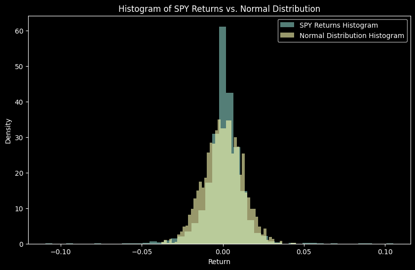
Another thing we could do aside from the volatility estimate, is the actual return distribution profile. So specifically, perhaps returns are not normally distributed.
spy = spy_daily

fig, ax = plt.subplots(figsize=(10, 6))
mean, scale = spy.mean(), spy.std()
normal_x = np.random.normal(loc=mean, scale=scale, size=len(spy))

ax.hist(spy, bins=50, density=True, alpha=0.6, label="SPY Returns Histogram")
ax.hist(
    normal_x,
    bins=50,
    density=True,
    alpha=0.6,
    label="Normal Distribution Histogram",
)
ax.set_title("Histogram of SPY Returns vs. Normal Distribution")
ax.set_xlabel("Return")
ax.set_ylabel("Density")
ax.legend()
plt.show()
KDE#
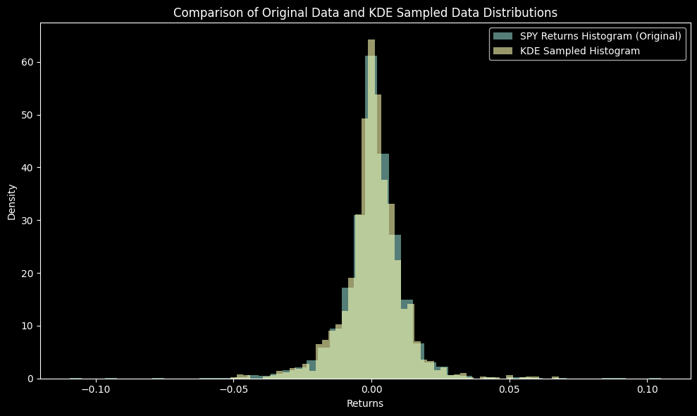
Therefore, we could do something like kernel density estimation (KDE) to “smooth” our return distribution and have a quasi-parametric VaR model.
Where we can think of each \(K\) as a bump (typically Gaussian), and some smoothing parameter \(h\) that controls how wide the bumps are. So basically treat each data point as a little Gaussian, and then add them all up to get a smooth distribution.
from sklearn.neighbors import KernelDensity

kde = KernelDensity(kernel="gaussian", bandwidth=0.001).fit(spy.values.reshape(-1, 1))

new_samples = kde.sample(n_samples=len(spy))

fig, ax = plt.subplots(figsize=(10, 6))

ax.hist(
    spy,
    bins=50,
    alpha=0.6,
    density=True,
    label="SPY Returns Histogram (Original)",
)
ax.hist(
    new_samples.flatten(),
    bins=50,
    alpha=0.6,
    density=True,
    label="KDE Sampled Histogram",
)

ax.set_title("Comparison of Original Data and KDE Sampled Data Distributions")
ax.set_xlabel("Returns")
ax.set_ylabel("Density")
ax.legend()
plt.tight_layout()
plt.show()
Monte Carlo Simulation#
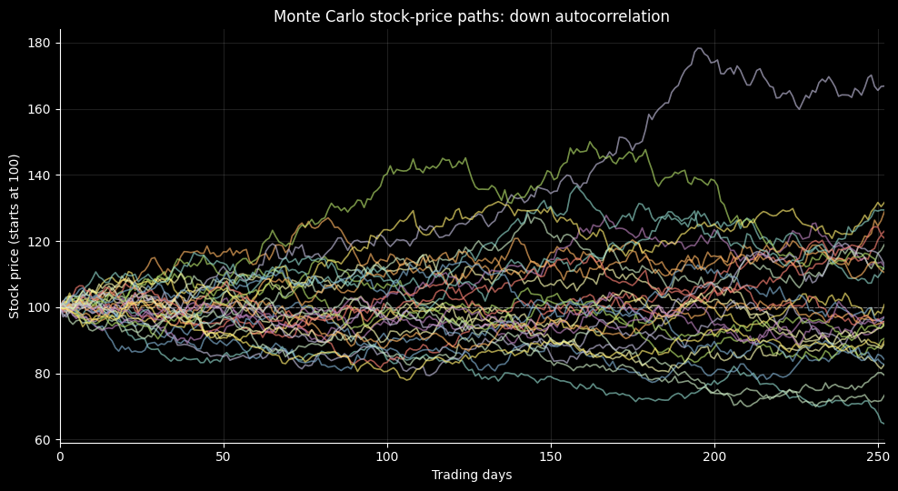
Now you can imagine potentially combining this with our previous volatility estimates.
Some other food for thought:
If we’re calculating the VaR for a portfolio, how do we account for correlations between assets?
How would persistence after negative returns affect the simulated tail?
Which additional dynamics would need empirical calibration?
Well, one easy way to do this would be to use a Monte Carlo simulation, where we can simulate a large number of return paths based on our volatility estimates, and then use the empirical distribution to calculate VaR. Simulation also would allow us to easily account for correlations between assets, path dynamics, etc.
The simulation below is an illustrative state-dependent process. Its 5% coefficient is assumed; it is not an estimate of SPY serial correlation.
log_spy = np.log1p(spy)
mu = log_spy.mean()
sigma = log_spy.std()
rng = np.random.default_rng(7)

N_PATHS = 10_000
N_DAYS_FORECAST = 252
DOWN_AUTOCORRELATION = 0.0

simulated_log_returns = np.zeros((N_DAYS_FORECAST, N_PATHS))
last_log_return = log_spy.iloc[-1]

for i in range(N_PATHS):
    current_log_return = last_log_return

    for t in range(N_DAYS_FORECAST):
        z = rng.normal(0, 1)
        unconditional_return = mu + sigma * z

        if current_log_return < 0:
            new_return = (DOWN_AUTOCORRELATION * current_log_return) + (
                (1 - DOWN_AUTOCORRELATION) * unconditional_return
            )
        else:
            new_return = unconditional_return

        simulated_log_returns[t, i] = new_return
        current_log_return = new_return

simulated_simple_returns = np.exp(simulated_log_returns) - 1
cumulative_returns = np.prod(1 + simulated_simple_returns, axis=0) - 1

VaR_level = 0.05
VaR_return = np.percentile(cumulative_returns, VaR_level * 100)
VaR_loss = -VaR_return

independent_cumulative_returns = cumulative_returns.copy()
rng = np.random.default_rng(7)
DOWN_AUTOCORRELATION = 0.05

simulated_log_returns = np.zeros((N_DAYS_FORECAST, N_PATHS))
last_log_return = log_spy.iloc[-1]

for i in range(N_PATHS):
    current_log_return = last_log_return

    for t in range(N_DAYS_FORECAST):
        z = rng.normal(0, 1)
        unconditional_return = mu + sigma * z

        if current_log_return < 0:
            new_return = (DOWN_AUTOCORRELATION * current_log_return) + (
                (1 - DOWN_AUTOCORRELATION) * unconditional_return
            )
        else:
            new_return = unconditional_return

        simulated_log_returns[t, i] = new_return
        current_log_return = new_return

simulated_simple_returns = np.exp(simulated_log_returns) - 1
cumulative_returns = np.prod(1 + simulated_simple_returns, axis=0) - 1

VaR_level = 0.05
VaR_return = np.percentile(cumulative_returns, VaR_level * 100)
VaR_loss = -VaR_return

mc_comparison = pd.DataFrame(
    {
        "Down autocorrelation": [0.0, DOWN_AUTOCORRELATION],
        "1-year return VaR (5%)": [
            np.quantile(independent_cumulative_returns, VaR_level),
            VaR_return,
        ],
    },
    index=["Independent returns", "Down autocorrelation"],
)
display(
    mc_comparison.style.format(
        {
            "Down autocorrelation": "{:.0%}",
            "1-year return VaR (5%)": "{:.2%}",
        }, na_rep="n/a"
    )
)

price_paths = 100 * np.exp(
    np.vstack([np.zeros((1, 30)), simulated_log_returns[:, :30].cumsum(axis=0)])
)
fig, ax = plt.subplots(figsize=(10, 5.5))
ax.plot(price_paths, linewidth=1.2, alpha=0.65)
ax.axhline(100, linestyle="--", linewidth=0.8, alpha=0.4)
ax.set(
    title="Monte Carlo stock-price paths: down autocorrelation",
    xlabel="Trading days",
    ylabel="Stock price (starts at 100)",
    xlim=(0, N_DAYS_FORECAST),
)
ax.grid(alpha=0.12)
ax.spines[["top", "right"]].set_visible(False)
fig.tight_layout()
plt.show()
| Down autocorrelation | 1-year return VaR (5%) | |
|---|---|---|
| Independent returns | 0% | -15.83% |
| Down autocorrelation | 5% | -20.65% |