


TA Review - CAPM#
TA: Tobias Rodriguez del Pozo
Autumn 2026. Thank you to Brian Wickman for his help with this notebook.
The industry examples use monthly excess returns from January 1980 through April 2025. The ETF examples use February 2011 through May 2025. Rerunning with updated course data can change the estimates.
See also Tobias Tip - CAPM.
import numpy as np
import pandas as pd
import statsmodels.api as sm
import matplotlib.pyplot as plt
from matplotlib.ticker import PercentFormatter
from IPython.display import display

plt.style.use("dark_background")
ANNUALIZATION = 12
factors = pd.read_excel(
    "../data/factor_pricing_data.xlsx",
    sheet_name="factors (excess returns)",
    index_col=0,
    parse_dates=True,
)
assets = pd.read_excel(
    "../data/factor_pricing_data.xlsx",
    sheet_name="portfolios (excess returns)",
    index_col=0,
    parse_dates=True,
)
assets.columns = assets.columns.str.strip()
panel = assets.join(factors[["MKT"]], how="inner").dropna().sort_index()
market = panel["MKT"]
assets = panel.drop(columns="MKT")
print(
    f"{assets.shape[1]} industry portfolios | Monthly excess returns | "
    f"{panel.index[0]:%b %Y}–{panel.index[-1]:%b %Y} | {len(panel)} observations"
)
49 industry portfolios | Monthly excess returns | Jan 1980–Apr 2025 | 544 observations
CAPM Introduction#
The central idea behind the CAPM is that it is a statement about expectations.
MV gives us how to construct an optimal portfolio given \(\mu\) and \(\Sigma\), but how might we get a better \(\mu\)? Well “asset pricing models” are one way to do this.
The CAPM states that expected return is a linear function of a single source of risk (market risk):
where
where \(\tilde{r}^i\) is the (excess) return of asset \(i\) and \(\tilde{r}^m\) is the (excess) return of the market portfolio. That is, the expected return of an asset is just directly proportional its market beta.
What is MSFT’s expected excess return?#
If MSFT has a beta of 1.2 and the expected excess return of the market portfolio is 8%, then MSFT’s expected excess return is:
Note that the CAPM takes the expected return of the market and risk-free rate as inputs. Thus, it is a relative pricing formula (relative to the inputs)…
The market portfolio is a value-weighted portfolio of all (not just equities) available assets, including the non-traded and illiquid. In practice, a broad equity index like SPY is used.
What does it mean for the CAPM beta to be negative?
The asset tends to move in the opposite direction of the market.
CAPM and Risk Premia#
Let’s look at the CAPM equation in depth:
With the assumption that \(\mathbb{E}[\varepsilon^i] = 0\) and \(\text{cov}(\varepsilon^i, \tilde{r}^m) = 0\) (these moment restrictions do not imply strict exogeneity).
For the variance, recall \(\text{Var}(aX)=a^2\text{Var}(X), \, \text{for } a\in\mathbb{R}\).
Define risk premium of an asset as the expected excess return of that asset over the risk-free rate.
CAPM states that the risk premium of an asset is proportional to the market risk premium (an equity risk premium when an equity index is used as the market proxy).
The only risk associated with higher expected returns is exposure to the market portfolio.
But we can be even more specific! Since the market portfolio is mean-variance efficient (idiosyncratic risk can be diversified away), only exposure to systematic risk is priced!
Investors should expect no additional compensation/ return for bearing idiosyncratic risk.
assumed_market_premium = 0.08
assumed_market_vol = 0.16
risk_examples = pd.DataFrame(
    {
        "Beta": [1.0, 1.0, 0.5, -0.5, 1.0],
        "Idiosyncratic volatility": [0.05, 0.30, 0.30, 0.05, 0.0],
    },
    index=["A", "B", "C", "Negative beta", "Market"],
)
risk_examples["Expected excess return"] = risk_examples["Beta"] * assumed_market_premium
risk_examples["Total volatility"] = np.sqrt(
    (risk_examples["Beta"] * assumed_market_vol) ** 2
    + risk_examples["Idiosyncratic volatility"] ** 2
)
risk_examples["Sharpe ratio"] = (
    risk_examples["Expected excess return"] / risk_examples["Total volatility"]
)
risk_examples.style.format(
    {
        "Beta": "{:.1f}",
        "Idiosyncratic volatility": "{:.1%}",
        "Expected excess return": "{:.1%}",
        "Total volatility": "{:.1%}",
        "Sharpe ratio": "{:.2f}",
    }
, na_rep="n/a").set_caption("CAPM examples: annual inputs and outputs")
| Beta | Idiosyncratic volatility | Expected excess return | Total volatility | Sharpe ratio | |
|---|---|---|---|---|---|
| A | 1.0 | 5.0% | 8.0% | 16.8% | 0.48 |
| B | 1.0 | 30.0% | 8.0% | 34.0% | 0.24 |
| C | 0.5 | 30.0% | 4.0% | 31.0% | 0.13 |
| Negative beta | -0.5 | 5.0% | -4.0% | 9.4% | -0.42 |
| Market | 1.0 | 0.0% | 8.0% | 16.0% | 0.50 |
CAPM and Sharpe Ratios#
Let’s see what the CAPM has to say about Sharpe Ratios (recall \(SR = \mathbb{E}[\tilde{r}^i]/\sigma^i\)):
The Sharpe Ratio of asset \(i\) is proportional to the Sharpe Ratio of the market portfolio, scaled by the correlation between asset \(i\) and the market portfolio.
Time-Series Test of the CAPM: Estimating Betas#
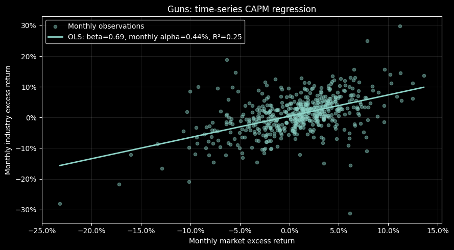
For any asset \(i\), run a time-series regression of excess returns \(i\) on the excess market return to estimate \(\alpha^i\) and \(\beta^{i,m}\):
The way that we can check this is using the standard t-test for the intercept term (in the case of a single asset regression). Recall from the Data Analysis and Regression reviews that the t-statistic for a coefficient is given by:
industry = "Guns"
fit = sm.OLS(assets[industry], sm.add_constant(market)).fit()
beta = fit.params["MKT"]
alpha = fit.params["const"]

fig, ax = plt.subplots(figsize=(9, 5))
ax.scatter(market, assets[industry], s=20, alpha=0.45, label="Monthly observations")
market_grid = np.linspace(market.min(), market.max(), 100)
ax.plot(
    market_grid,
    alpha + beta * market_grid,
    linewidth=2,
    label=f"OLS: beta={beta:.2f}, monthly alpha={alpha:.2%}, R²={fit.rsquared:.2f}",
)
ax.set(
    title=f"{industry}: time-series CAPM regression",
    xlabel="Monthly market excess return",
    ylabel="Monthly industry excess return",
)
ax.xaxis.set_major_formatter(PercentFormatter(1))
ax.yaxis.set_major_formatter(PercentFormatter(1))
ax.legend()
ax.grid(alpha=0.12)
fig.tight_layout()
plt.show()
industry_fits = {
    name: sm.OLS(assets[name], sm.add_constant(market)).fit() for name in assets
}
industry_metrics = pd.DataFrame(
    {
        name: {
            "Beta": result.params["MKT"],
            "Annual alpha": result.params["const"] * ANNUALIZATION,
            "Alpha t-stat": result.tvalues["const"],
            "Alpha p-value": result.pvalues["const"],
            "Time-series R²": result.rsquared,
        }
        for name, result in industry_fits.items()
    }
).T
industry_metrics.loc[["Guns", "Util", "Softw", "Oil", "Food", "Banks"]].style.format(
    {
        "Beta": "{:.2f}",
        "Annual alpha": "{:.2%}",
        "Alpha t-stat": "{:.2f}",
        "Alpha p-value": "{:.3f}",
        "Time-series R²": "{:.3f}",
    }
, na_rep="n/a").set_caption("Individual alpha tests: conventional OLS standard errors")
| Beta | Annual alpha | Alpha t-stat | Alpha p-value | Time-series R² | |
|---|---|---|---|---|---|
| Guns | 0.69 | 5.24% | 1.84 | 0.066 | 0.248 |
| Util | 0.46 | 3.70% | 2.08 | 0.038 | 0.273 |
| Softw | 1.36 | 2.01% | 0.81 | 0.417 | 0.626 |
| Oil | 0.86 | 0.89% | 0.33 | 0.743 | 0.358 |
| Food | 0.58 | 4.26% | 2.36 | 0.019 | 0.360 |
| Banks | 1.07 | 0.10% | 0.05 | 0.962 | 0.612 |
Multiple testing#
We need to be very careful about multiple hypothesis testing.
There are two main ways to deal with this:
Bonferroni correction: Divide the significance level by the number of tests. This is conservative.
Benjamini-Hochberg (BH): This algorithm controls the false discovery rate (FDR) by ranking the p-values and comparing them to a threshold that increases with the rank. This allows us to control the expected proportion of false discoveries among significant results (under independence or suitable positive dependence).
from statsmodels.stats.multitest import multipletests

significance = 0.05
alpha_tests = (
    industry_metrics[["Annual alpha", "Alpha p-value"]]
    .rename(columns={"Alpha p-value": "Raw p-value"})
    .copy()
)
raw_pvalues = alpha_tests["Raw p-value"]
bh_reject, alpha_tests["BH p-value"], _, _ = multipletests(
    raw_pvalues, alpha=significance, method="fdr_bh"
)
bonf_reject, alpha_tests["Bonferroni p-value"], _, _ = multipletests(
    raw_pvalues, alpha=significance, method="bonferroni"
)
display(
    alpha_tests.sort_values("Raw p-value")
    .head(8)
    .style.format(
        {
            "Annual alpha": "{:.2%}",
            "Raw p-value": "{:.4f}",
            "BH p-value": "{:.4f}",
            "Bonferroni p-value": "{:.4f}",
        }
    , na_rep="n/a")
    .set_caption(
        f"Eight smallest raw p-values; adjustments use all {len(alpha_tests)} industries"
    )
)

rejection_counts = pd.DataFrame(
    {
        "Error criterion": [
            "Per-test error",
            "False discovery rate",
            "Family-wise error",
        ],
        "Tests": len(alpha_tests),
        "Rejected at 5%": [
            (raw_pvalues < significance).sum(),
            bh_reject.sum(),
            bonf_reject.sum(),
        ],
    },
    index=["Unadjusted", "BH", "Bonferroni"],
)
display(rejection_counts.style.format({"Error criterion": "{}", "Tests": "{:.0f}", "Rejected at 5%": "{:.0f}"}, na_rep="n/a"))
| Annual alpha | Raw p-value | BH p-value | Bonferroni p-value | |
|---|---|---|---|---|
| Smoke | 8.80% | 0.0040 | 0.1937 | 0.1937 |
| Beer | 5.34% | 0.0112 | 0.2749 | 0.5499 |
| Food | 4.26% | 0.0186 | 0.3045 | 0.9136 |
| Drugs | 3.87% | 0.0288 | 0.3387 | 1.0000 |
| Util | 3.70% | 0.0379 | 0.3387 | 1.0000 |
| Steel | -5.79% | 0.0415 | 0.3387 | 1.0000 |
| Rtail | 3.07% | 0.0597 | 0.3918 | 1.0000 |
| Guns | 5.24% | 0.0656 | 0.3918 | 1.0000 |
| Error criterion | Tests | Rejected at 5% | |
|---|---|---|---|
| Unadjusted | Per-test error | 49 | 6 |
| BH | False discovery rate | 49 | 0 |
| Bonferroni | Family-wise error | 49 | 0 |
Joint Test of Alphas#
For a fixed set of \(n\) assets and \(T\) observations, assume independent, identically distributed jointly normal returns and a nonsingular residual covariance matrix. We can test the joint null that all alphas are zero using the asymptotic statistic below. Alphas, the market Sharpe ratio, and the residual covariance matrix must use the same return frequency.
This is a large-sample chi-square test. Its p-value is not the finite-sample GRS F-test p-value.
from scipy.stats import chi2

monthly_alphas = pd.Series(
    {name: result.params["const"] for name, result in industry_fits.items()}
)
capm_residuals = pd.DataFrame(
    {name: result.resid for name, result in industry_fits.items()}
)
T, n = capm_residuals.shape
market_sharpe_monthly = market.mean() / market.std()

H = (
    T
    / (1 + market_sharpe_monthly**2)
    * (monthly_alphas @ np.linalg.solve(capm_residuals.cov(), monthly_alphas))
)
joint_pvalue = chi2.sf(H, df=n)

pd.DataFrame(
    {
        "H": [H],
        "Degrees of freedom": [n],
        "p-value": [joint_pvalue],
        "Reject at 5%": [joint_pvalue < 0.05],
    },
    index=["All alphas = 0"],
).style.format({"H": "{:.2f}", "Degrees of freedom": "{:.0f}", "p-value": "{:.3f}", "Reject at 5%": "{}"}, na_rep="n/a")
| H | Degrees of freedom | p-value | Reject at 5% | |
|---|---|---|---|---|
| All alphas = 0 | 62.98 | 49 | 0.087 | False |
The CAPM restricts the population alphas to zero. It imposes no requirement that the time-series regressions have high \(R^2\).
Residual variance still affects the standard error of the estimated alpha. Holding the market observations and sample size fixed, more residual variance makes a given alpha harder to distinguish from zero.
rng = np.random.default_rng(21)
market_sim = pd.Series(rng.normal(0.006, 0.04, 240), name="Market")
shock = rng.normal(size=len(market_sim))
simulation_rows = []
for true_alpha, residual_vol in [(0, 0.01), (0, 0.08), (0.004, 0.01), (0.004, 0.08)]:
    simulated_return = true_alpha + market_sim + residual_vol * shock
    result = sm.OLS(simulated_return, sm.add_constant(market_sim)).fit()
    simulation_rows.append(
        {
            "True annual alpha": true_alpha * ANNUALIZATION,
            "Fitted annual alpha": result.params["const"] * ANNUALIZATION,
            "Residual vol (annual)": residual_vol * np.sqrt(ANNUALIZATION),
            "Alpha SE (annual)": result.bse["const"] * ANNUALIZATION,
            "Alpha p-value": result.pvalues["const"],
            "Time-series R²": result.rsquared,
        }
    )
simulation_table = pd.DataFrame(simulation_rows, index=["A", "B", "C", "D"])
simulation_table.style.format(
    {
        "True annual alpha": "{:.2%}",
        "Fitted annual alpha": "{:.2%}",
        "Residual vol (annual)": "{:.1%}",
        "Alpha SE (annual)": "{:.2%}",
        "Alpha p-value": "{:.3f}",
        "Time-series R²": "{:.3f}",
    }
, na_rep="n/a").set_caption(
    "Simulated monthly returns: beta=1, 240 observations, common random draws"
)
| True annual alpha | Fitted annual alpha | Residual vol (annual) | Alpha SE (annual) | Alpha p-value | Time-series R² | |
|---|---|---|---|---|---|---|
| A | 0.00% | 0.97% | 3.5% | 0.74% | 0.191 | 0.938 |
| B | 0.00% | 7.76% | 27.7% | 5.91% | 0.191 | 0.192 |
| C | 4.80% | 5.77% | 3.5% | 0.74% | 0.000 | 0.938 |
| D | 4.80% | 12.56% | 27.7% | 5.91% | 0.035 | 0.192 |
Cross-Sectional Test of the CAPM#
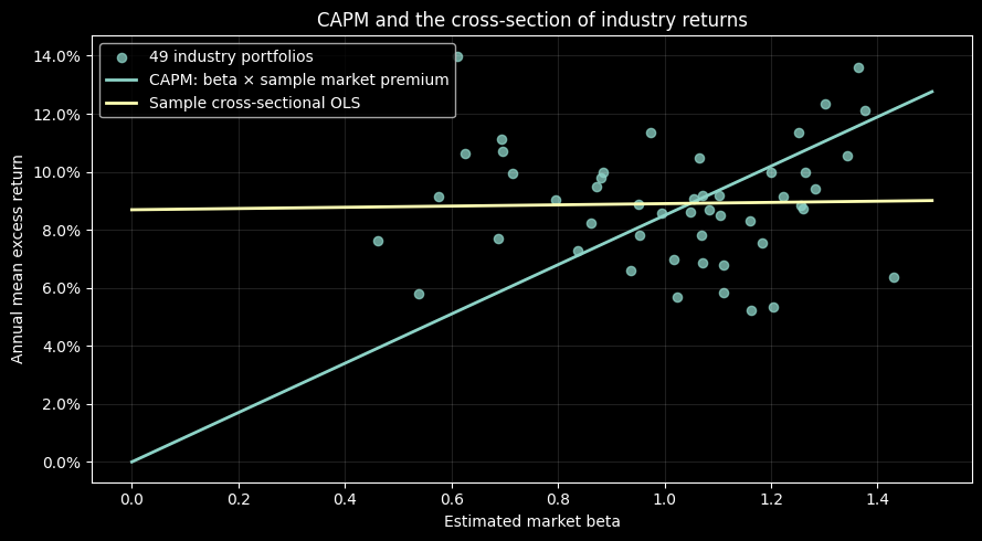
We collect a large number of assets, and for each asset, we estimate its market beta by regressing its returns against market returns (with an intercept). Then, we take the estimated betas and run a cross-sectional regression of average asset returns against their estimated betas. The CAPM predicts that the slope of this regression should be equal to the expected market risk premium.
where \(\lambda_m\) is the amount of risk premium an asset gets per unit of market beta or the price of risk!
Estimate each asset’s market beta \(\beta^{i,m}\) from a time-series regression of excess returns on excess market returns. Use the estimated betas as regressors in the second stage. Formal inference must account for their estimation error and dependence across asset returns; the calculation below is descriptive.
Run a cross-sectional regression of average excess returns on estimated market betas:
Notes
The cross-sectional regression estimates the intercept \(\eta\) and slope \(\lambda_m\), not the market betas.
This is not a time-series regression (no \(t\) subscripts).
cross_section = pd.DataFrame(
    {
        "Mean excess return": assets.mean() * ANNUALIZATION,
        "Beta": industry_metrics["Beta"],
    }
)
cross_fit = sm.OLS(
    cross_section["Mean excess return"], sm.add_constant(cross_section["Beta"])
).fit()
sample_market_premium = market.mean() * ANNUALIZATION
beta_grid = np.linspace(0, cross_section["Beta"].max() * 1.05, 100)

fig, ax = plt.subplots(figsize=(9, 5))
ax.scatter(
    cross_section["Beta"],
    cross_section["Mean excess return"],
    s=35,
    alpha=0.75,
    label="49 industry portfolios",
)
ax.plot(
    beta_grid,
    sample_market_premium * beta_grid,
    label="CAPM: beta × sample market premium",
    linewidth=2,
)
ax.plot(
    beta_grid,
    cross_fit.params["const"] + cross_fit.params["Beta"] * beta_grid,
    label="Sample cross-sectional OLS",
    linewidth=2,
)
ax.set(
    xlabel="Estimated market beta",
    ylabel="Annual mean excess return",
    title="CAPM and the cross-section of industry returns",
)
ax.yaxis.set_major_formatter(PercentFormatter(1))
ax.legend()
ax.grid(alpha=0.12)
fig.tight_layout()
plt.show()

cross_summary = pd.DataFrame(
    {
        "Annual intercept": [cross_fit.params["const"]],
        "Annual slope": [cross_fit.params["Beta"]],
        "Sample market premium": [sample_market_premium],
        "Sample cross-sectional R²": [cross_fit.rsquared],
    },
    index=["Sample estimates"],
)
cross_summary.style.format(
    {
        "Annual intercept": "{:.2%}",
        "Annual slope": "{:.2%}",
        "Sample market premium": "{:.2%}",
        "Sample cross-sectional R²": "{:.3f}",
    }
, na_rep="n/a")
| Annual intercept | Annual slope | Sample market premium | Sample cross-sectional R² | |
|---|---|---|---|---|
| Sample estimates | 8.69% | 0.21% | 8.49% | 0.001 |
Population Restrictions#
If the CAPM were completely accurate (population restrictions):
Intercept |
\(R^2\) |
\(\varepsilon^i\) / \(\nu^i\) |
\(\lambda_m\) (Price of risk) |
|
|---|---|---|---|---|
Time Series |
0 |
\(0\le R^2\le 1\) |
\(\mathbb{E}[\varepsilon^i]=0\) |
|
Cross-Sectional |
0 |
1 |
0 |
\(\mathbb{E}\left[\tilde{r}^m\right]\) |
CAPM predicts expected returns, but realized returns can deviate significantly in small samples due to random fluctuations.
Sample Midterm Question#
Which of the following two stocks has the higher expected return according to the CAPM?
AI Chip Manufacturer |
Public Utility |
|
|---|---|---|
Historical average return |
15% |
5% |
Volatility |
35% |
10% |
Value at Risk (VaR) |
-10% |
-3% |
Not enough information to tell.
Expected and realized returns#
Here’s the statistical equivalent of CAPM on single-year returns (or small samples):
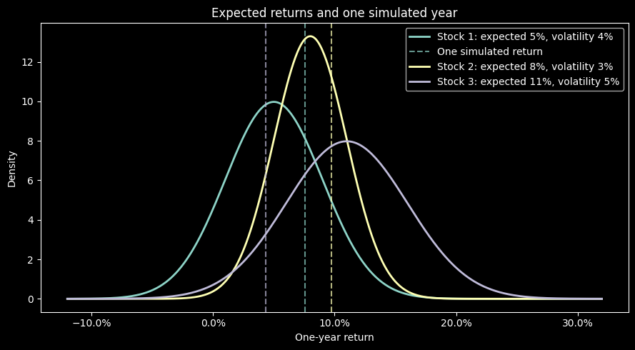
Consider three stocks with normally-distributed returns \(\sim N(\mu, \sigma^2)\), with \((\mu,\sigma)\): (0.05, 0.04), (0.08, 0.03), (0.11, 0.05).
The returns have different means and variances, but there is a lot of overlap between them
In a single draw from each distribution, it is quite possible that the draw from the lowest-mean distribution is higher than the draw from the highest-mean distribution.
CAPM makes a statement about expected excess return, but the high variance of stock returns (particularly idiosyncratic risk) makes it difficult to observe the expected return ordering predicted by CAPM in a single year. Use the Time-Series, Cross-Sectional regressions to formally test CAPM (and other factor models)!
from scipy.stats import norm

brian_rng = np.random.RandomState(42)
distribution_params = [(0.05, 0.04), (0.08, 0.03), (0.11, 0.05)]
samples = [brian_rng.normal(mu, sigma, 100_000) for mu, sigma in distribution_params]
single_draws = [sample[2] for sample in samples]
display(
    pd.DataFrame(
        {
            "Expected return": [mu for mu, sigma in distribution_params],
            "Volatility": [sigma for mu, sigma in distribution_params],
            "One simulated return": single_draws,
        },
        index=["Stock 1", "Stock 2", "Stock 3"],
    ).style.format({"Expected return": "{:.2%}", "Volatility": "{:.2%}", "One simulated return": "{:.2%}"}, na_rep="n/a")
)

return_grid = np.linspace(-0.12, 0.32, 500)
fig, ax = plt.subplots(figsize=(9, 5))
for i, ((mu, sigma), realized) in enumerate(zip(distribution_params, single_draws), 1):
    (line,) = ax.plot(
        return_grid,
        norm.pdf(return_grid, mu, sigma),
        linewidth=2,
        label=f"Stock {i}: expected {mu:.0%}, volatility {sigma:.0%}",
    )
    ax.axvline(
        realized,
        linestyle="--",
        alpha=0.7,
        color=line.get_color(),
        label="One simulated return" if i == 1 else None,
    )
ax.set(
    title="Expected returns and one simulated year",
    xlabel="One-year return",
    ylabel="Density",
)
ax.xaxis.set_major_formatter(PercentFormatter(1))
ax.legend()
fig.tight_layout()
plt.show()
| Expected return | Volatility | One simulated return | |
|---|---|---|---|
| Stock 1 | 5.00% | 4.00% | 7.59% |
| Stock 2 | 8.00% | 3.00% | 9.73% |
| Stock 3 | 11.00% | 5.00% | 4.35% |
Market Beta, Information Ratio and Treynor Ratio#
Downside beta conditions on negative market excess returns:
Which regresses the returns of the asset on the returns of the market, but only when the market is down. This is a measure of the systematic downside risk of the asset. Why might this be more useful in a hedge fund setting?
Information ratio:
Treynor ratio:
etfs = pd.read_excel(
    "../data/multi_asset_etf_data.xlsx",
    sheet_name="excess returns",
    index_col=0,
    parse_dates=True,
)[["SPY", "PSP", "HYG", "IYR"]].dropna()
print(f"Monthly excess returns: {etfs.index[0]:%b %Y}–{etfs.index[-1]:%b %Y}")
extra_rows = {}
for ticker in ["PSP", "HYG", "IYR"]:
    result = sm.OLS(etfs[ticker], sm.add_constant(etfs["SPY"])).fit()
    down = etfs.loc[etfs["SPY"] < 0]
    down_result = sm.OLS(down[ticker], sm.add_constant(down["SPY"])).fit()
    extra_rows[ticker] = {
        "Beta": result.params["SPY"],
        "Downside beta": down_result.params["SPY"],
        "Annual alpha": result.params["const"] * ANNUALIZATION,
        "Information ratio": result.params["const"]
        / result.resid.std()
        * np.sqrt(ANNUALIZATION),
        "Treynor ratio (annual)": etfs[ticker].mean()
        * ANNUALIZATION
        / result.params["SPY"],
    }
pd.DataFrame(extra_rows).T.style.format(
    {
        "Beta": "{:.2f}",
        "Downside beta": "{:.2f}",
        "Annual alpha": "{:.2%}",
        "Information ratio": "{:.2f}",
        "Treynor ratio (annual)": "{:.2%}",
    }
, na_rep="n/a").set_caption("Benchmark: SPY; monthly excess returns")
Monthly excess returns: Feb 2011–May 2025
| Beta | Downside beta | Annual alpha | Information ratio | Treynor ratio (annual) | |
|---|---|---|---|---|---|
| PSP | 1.33 | 1.50 | -7.81% | -0.81 | 6.95% |
| HYG | 0.42 | 0.52 | -1.27% | -0.27 | 9.81% |
| IYR | 0.89 | 1.07 | -3.93% | -0.36 | 8.41% |
Market Volatility and Asset Correlations#
A one-factor return model can produce rising correlations when market volatility rises. This is a covariance result under additional assumptions, rather than an implication of the CAPM expected-return restriction alone. Consider two assets \(i\) and \(j\):
Now, let’s consider the covariances between the two assets, assuming idiosyncratic risks are uncorrelated \(\text{cov}(\varepsilon^i, \varepsilon^j) = 0\), we have:
Assuming both \(\beta\)’s are positive, with fixed betas and idiosyncratic variances:
For low market volatility, the idiosyncratic terms dominate.
For high market volatility, market-wide shocks overwhelm idiosyncratic noise, and assets move together, increasing correlation.