


MV of S&P 500#
How does mean-variance optimization behave as the universe grows?
Data - weekly returns for 503 S&P 500 names, 2015 to 2026.
Nested subsamples - draw 5 names at random, then 20 containing those 5, and so on up to the full panel.
Three numbers per \(\Nsec\) - best single-name Sharpe, tangency Sharpe, gross position size.
Caveat: the panel is current members with full ten-year histories. Survivorship tilts every statistic here upward.
import numpy as np
import pandas as pd
pd.options.display.float_format = "{:,.4f}".format

import matplotlib.pyplot as plt
import seaborn as sns

import statsmodels.api as sm
from sklearn.linear_model import LinearRegression
filepath_data = '../data/spx_returns_weekly.xlsx'
SHEET = 'spx returns'
rets_raw = pd.read_excel(filepath_data,sheet_name=SHEET).set_index('date')
print(f'{rets_raw.shape[1]} names, weekly, {rets_raw.index[0]:%b %Y} to {rets_raw.index[-1]:%b %Y}')
503 names, weekly, Jul 2015 to Jul 2026
FREQ = 52 # weekly data (spx_returns_weekly)
Frontiers by N#
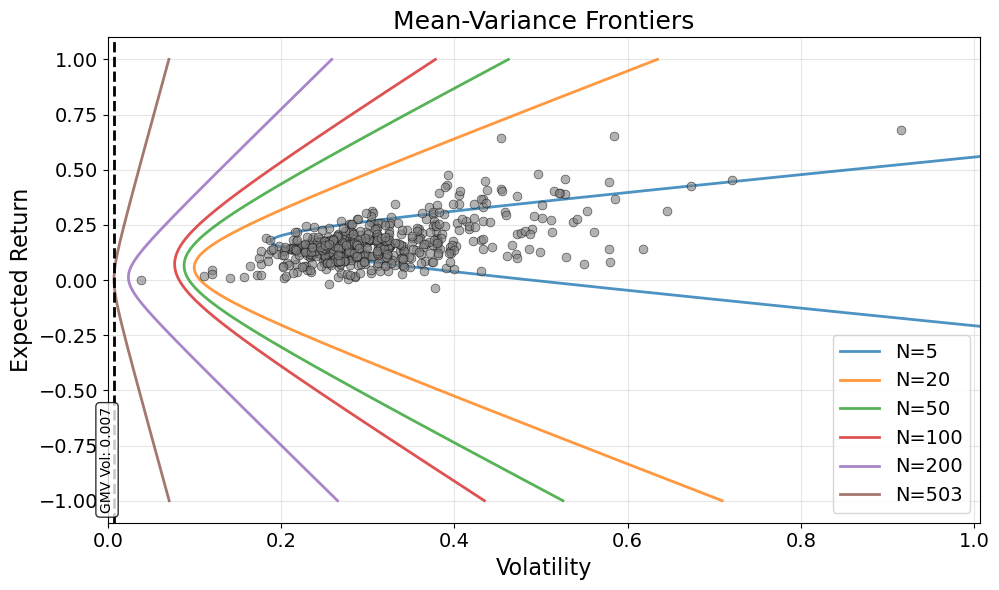
One frontier per nested subsample; dots are individual names.
Adding names never hurts: the frontier weakly expands with \(\Nsec\).
# Multi-Frontier Plot for Various N Values (Nested Subsamples)
N_values = [5, 20, 50, 100, 200, len(rets_raw.columns)]

fig, ax = plt.subplots(figsize=(10, 6))

# Create nested subsamples
np.random.seed(2025)  # Use same seed for reproducibility
all_assets = list(rets_raw.columns)
np.random.shuffle(all_assets)  # Shuffle once for consistent ordering

# Track which assets are included at each N level
asset_inclusion_level = {}
nested_asset_sets = {}

# Initialize summary data storage
summary_data = []

# Create nested sets
for i, N in enumerate(N_values):
    if N > len(rets_raw.columns):
        continue  # Skip if N is larger than available assets

    # For the first N, take the first N assets
    # For subsequent N values, take the previous assets plus additional ones
    if i == 0:
        selected_assets = all_assets[:N]
    else:
        # Take all assets from previous levels plus additional ones
        selected_assets = nested_asset_sets[N_values[i-1]] + all_assets[len(nested_asset_sets[N_values[i-1]]):N]

    nested_asset_sets[N] = selected_assets
    idx = sorted(selected_assets)
    rets_n = rets_raw[idx]

    # Track which N level each asset was first included in
    for asset in selected_assets:
        if asset not in asset_inclusion_level:
            asset_inclusion_level[asset] = N

    # Calculate metrics for this N
    mu_n = rets_n.mean() * FREQ
    covmat_n = rets_n.cov() * FREQ
    vec_ones_n = np.ones(mu_n.shape)

    # Calculate GMV and tangency portfolios
    w_gmv_n = np.linalg.solve(covmat_n, vec_ones_n)
    w_tan_n = np.linalg.solve(covmat_n, mu_n)
    w_gmv_n /= w_gmv_n.sum()
    w_tan_n /= w_tan_n.sum()

    # Calculate Sharpe ratios and gross market value for this N
    # Individual asset Sharpe ratios
    individual_sharpe = mu_n / (rets_n.std() * np.sqrt(FREQ))
    max_individual_sharpe = individual_sharpe.max()

    # Tangency portfolio Sharpe ratio
    tangency_sharpe = (mu_n.T @ w_tan_n) / np.sqrt(w_tan_n.T @ covmat_n @ w_tan_n)

    # Gross market value of tangency portfolio
    gross_market_value = np.abs(w_tan_n).sum()

    # Store summary data
    summary_data.append({
        'N': N,
        'Max_Individual_Sharpe': max_individual_sharpe,
        'Tangency_Sharpe': tangency_sharpe,
        'Gross_Market_Value': gross_market_value
    })

    # Define delta parameter function for this N
    def delta_parameter_n(target_mean):
        delta = (target_mean - mu_n.T@w_gmv_n)/(mu_n.T@w_tan_n - mu_n.T@w_gmv_n)
        return delta

    # Create frontier for this N
    MAX_n = (N+5) * .0005 * FREQ
    MIN_n = - MAX_n/1.6
    MAX_n = -1
    MIN_n = 1

    grid_n = np.linspace(MIN_n, MAX_n, 250)
    df_n = pd.DataFrame(index=grid_n, columns=['delta','mu','vol'], dtype=float)

    for mu_target in grid_n:
        delta = delta_parameter_n(mu_target)
        w = delta * w_tan_n + (1-delta) * w_gmv_n
        df_n.loc[mu_target,'delta'] = delta
        df_n.loc[mu_target,'mu'] = w.T @ mu_n
        df_n.loc[mu_target,'vol'] = np.sqrt(w.T @ covmat_n @ w)

    # Plot this frontier
    ax.plot(df_n['vol'], df_n['mu'],
            linewidth=2, alpha=0.8, label=f'N={N}')

# Plot base assets colored by inclusion level
base_mu = rets_raw.mean() * FREQ
base_vol = rets_raw.std() * np.sqrt(FREQ)

# Create color mapping for assets based on their first inclusion level
for N in N_values:
    if N > len(rets_raw.columns):
        continue

    # Get assets that were first included at this N level
    assets_at_level = [asset for asset, level in asset_inclusion_level.items() if level == N]

    if assets_at_level:
        # Get the corresponding mu and vol for these assets
        mu_at_level = base_mu[assets_at_level]
        vol_at_level = base_vol[assets_at_level]

        ax.scatter(vol_at_level, mu_at_level,
                  color='gray', alpha=0.6, s=40,
                  zorder=5, edgecolors='black', linewidth=0.5)

# Add vertical line at the global minimum variance portfolio of the largest N
largest_N = N_values[-1]
if largest_N <= len(rets_raw.columns):
    # Get the assets for the largest N
    largest_assets = nested_asset_sets[largest_N]
    largest_rets = rets_raw[largest_assets]

    # Calculate GMV portfolio for largest N
    largest_mu = largest_rets.mean() * FREQ
    largest_covmat = largest_rets.cov() * FREQ
    largest_vec_ones = np.ones(largest_mu.shape)
    largest_w_gmv = np.linalg.solve(largest_covmat, largest_vec_ones)
    largest_w_gmv /= largest_w_gmv.sum()

    # Calculate volatility of GMV portfolio
    gmv_vol = np.sqrt(largest_w_gmv.T @ largest_covmat @ largest_w_gmv)

    # Add vertical line
    ax.axvline(x=gmv_vol, color='black', linestyle='--', linewidth=2)

    # Add text label on x-axis
    ax.text(gmv_vol, ax.get_ylim()[0] + 0.02 * (ax.get_ylim()[1] - ax.get_ylim()[0]),
            f'GMV Vol: {gmv_vol:.3f}',
            rotation=90, verticalalignment='bottom', horizontalalignment='right',
            fontsize=10, bbox=dict(boxstyle='round,pad=0.3', facecolor='white', alpha=0.8))

ax.set_xlabel('Volatility', fontsize=16)
ax.set_ylabel('Expected Return', fontsize=16)
ax.set_title('Mean-Variance Frontiers', fontsize=18)
ax.legend(fontsize=14)
ax.grid(True, alpha=0.3)

# Increase tick label font sizes
ax.tick_params(axis='x', labelsize=14)
ax.tick_params(axis='y', labelsize=14)

plt.tight_layout()
ax.set_xlim(0, base_vol.max() * 1.1)
plt.show()
# Summary Table: Sharpe Ratios and Gross Market Values by N
summary_df = pd.DataFrame(summary_data)
summary_df = summary_df.set_index('N')

# Format the display
pd.options.display.float_format = "{:,.4f}".format

summary_df.style.format({
    'Max_Individual_Sharpe': "{:,.1%}",
    'Tangency_Sharpe': "{:,.1%}",
    'Gross_Market_Value': "{:,.1%}"
})
| Max_Individual_Sharpe | Tangency_Sharpe | Gross_Market_Value | |
|---|---|---|---|
| N | |||
| 5 | 93.0% | 100.8% | 115.1% |
| 20 | 99.1% | 161.0% | 345.2% |
| 50 | 103.2% | 219.0% | 669.0% |
| 100 | 103.4% | 267.6% | 940.3% |
| 200 | 142.0% | 387.5% | 1,392.3% |
| 503 | 142.0% | 1,425.4% | 28,304.3% |
Correlation Structure#
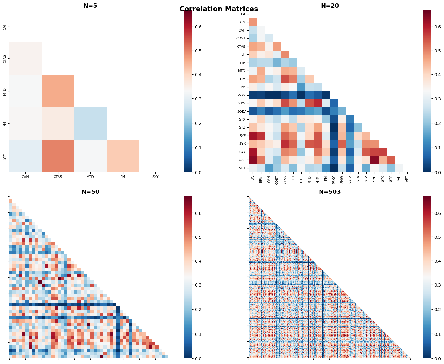
Diversification comes from imperfect correlation. Fragility comes from near-duplicates.
The condition number grows with \(\Nsec\): \(\covmat\) stays invertible, but barely, and \(\covmat^{-1}\) amplifies estimation noise.
# 2x2 Correlation Heatmaps for Various Subsets
from matplotlib.colors import TwoSlopeNorm

# Define subsets to analyze - smallest 3 N values and largest N
N_values_sorted = sorted([5, 20, 50, 100, len(rets_raw.columns)])
subset_configs = [
    {'name': f'N={N_values_sorted[0]}', 'size': N_values_sorted[0], 'title': f'N={N_values_sorted[0]}'},
    {'name': f'N={N_values_sorted[1]}', 'size': N_values_sorted[1], 'title': f'N={N_values_sorted[1]}'},
    {'name': f'N={N_values_sorted[2]}', 'size': N_values_sorted[2], 'title': f'N={N_values_sorted[2]}'},
    {'name': f'N={N_values_sorted[-1]}', 'size': N_values_sorted[-1], 'title': f'N={N_values_sorted[-1]}'}
]

# Use the same random seed for consistency
np.random.seed(2025)
all_assets = list(rets_raw.columns)
np.random.shuffle(all_assets)

fig, axes = plt.subplots(2, 2, figsize=(16, 12))
axes = axes.flatten()

for i, config in enumerate(subset_configs):
    # Select assets for this subset
    selected_assets = sorted(all_assets[:config['size']])
    rets_subset = rets_raw[selected_assets]

    # Calculate correlation matrix
    corr_matrix = rets_subset.corr()

    # Set upper triangle and diagonal to NaN for cleaner visualization
    mask = np.triu(np.ones_like(corr_matrix), k=0)
    corr_matrix_masked = corr_matrix.copy()
    corr_matrix_masked[mask.astype(bool)] = np.nan

    # Set up color normalization
    center = 0.33
    vmin = 0
    vmax = 0.67
    norm = TwoSlopeNorm(vmin=vmin, vcenter=center, vmax=vmax)

    # Create heatmap
    sns.heatmap(corr_matrix_masked,
                annot=False,  # No annotations
                norm=norm,
                cmap='RdBu_r',
                cbar=True,
                ax=axes[i],
                square=True)

    axes[i].set_title(config['title'], fontsize=14, fontweight='bold')

    # Adjust tick labels for readability
    if config['size'] <= 20:
        axes[i].tick_params(axis='both', labelsize=8)
    else:
        axes[i].tick_params(axis='both', labelsize=6)
        # For larger matrices, show fewer tick labels
        step = max(1, config['size'] // 10)
        axes[i].set_xticks(range(0, config['size'], step))
        axes[i].set_yticks(range(0, config['size'], step))

plt.tight_layout()
plt.suptitle('Correlation Matrices',
             fontsize=16, fontweight='bold', y=0.98)
plt.show()
# Correlation Statistics DataFrame
correlation_stats = []

# Use the same random seed for consistency
np.random.seed(2025)
all_assets = list(rets_raw.columns)
np.random.shuffle(all_assets)

for config in subset_configs:
    # Select assets for this subset
    selected_assets = sorted(all_assets[:config['size']])
    rets_subset = rets_raw[selected_assets]

    # Calculate correlation matrix
    corr_matrix = rets_subset.corr()

    # Calculate correlation statistics (excluding diagonal)
    mask = np.triu(np.ones_like(corr_matrix), k=1)
    correlations = corr_matrix.values[mask.astype(bool)]
    avg_pairwise_corr = correlations.mean()
    min_corr = correlations.min()
    max_corr = correlations.max()

    # Calculate condition number and determinant of correlation matrix
    condition_number = np.linalg.cond(corr_matrix)
    sign, logdet = np.linalg.slogdet(corr_matrix)
    log10_det = logdet / np.log(10)

    correlation_stats.append({
        'N': config['size'],
        'Min Correlation': min_corr,
        'Max Correlation': max_corr,
        'Avg Pairwise Correlation': avg_pairwise_corr,
        'Condition Number': condition_number,
        'log10 Determinant': log10_det
    })

# Create DataFrame
correlation_df = pd.DataFrame(correlation_stats)
correlation_df = correlation_df.set_index('N')
# Format the display
display_df = correlation_df.copy()
display_df['Min Correlation'] = display_df['Min Correlation'].apply(lambda x: f"{x:.0%}")
display_df['Max Correlation'] = display_df['Max Correlation'].apply(lambda x: f"{x:.0%}")
display_df['Avg Pairwise Correlation'] = display_df['Avg Pairwise Correlation'].apply(lambda x: f"{x:.0%}")
display_df['Condition Number'] = display_df['Condition Number'].apply(lambda x: f"{x:,.0f}")
display_df['log10 Determinant'] = display_df['log10 Determinant'].apply(lambda x: f"{x:,.0f}")

display_df
| Min Correlation | Max Correlation | Avg Pairwise Correlation | Condition Number | log10 Determinant | |
|---|---|---|---|---|---|
| N | |||||
| 5 | 25% | 50% | 36% | 5 | -0 |
| 20 | -2% | 64% | 31% | 27 | -3 |
| 50 | -4% | 80% | 31% | 117 | -13 |
| 503 | -32% | 100% | 32% | 479,647 | -385 |
Extreme Pairs#
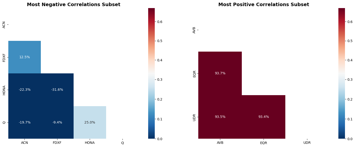
The most correlated distinct companies are same-sector near-duplicates: apartment REITs (AvalonBay, Equity Residential, UDR) and regulated utilities that share the same rate sensitivity and cash-flow profile.
Distinct firms, but nearly the same business - so the optimizer spread-trades them, driving the gross leverage.
A firm’s own share classes (GOOG/GOOGL, FOX/FOXA) correlate ~99% mechanically. Those are not distinct entities and are listed separately below.
# Correlation Heatmaps for Most Negative and Most Positive Pairs
from matplotlib.colors import TwoSlopeNorm
import re

# Ticker -> company, to spot a firm's own share classes (GOOG/GOOGL, FOX/FOXA)
ticker_mapping = pd.read_excel(filepath_data, sheet_name='spx names')
ticker_to_name = dict(zip(ticker_mapping.iloc[:, 0], ticker_mapping.iloc[:, 1]))
ticker_to_sector = dict(zip(ticker_mapping['ticker'], ticker_mapping['gics_sector_name']))

def name_root(nm):
    nm = re.sub(r'\s*[-/]\s*(CL|CLASS)\s+[A-C]\b', '', str(nm), flags=re.I)
    nm = re.sub(r'\b(inc|corp|co|ltd|plc|group|holdings|the)\b\.?', '', nm, flags=re.I)
    return re.sub(r'[^a-z0-9]', '', nm.lower())

def same_company(a, b):
    return name_root(ticker_to_name.get(a, a)) == name_root(ticker_to_name.get(b, b))

full_corr_matrix = rets_raw.corr()

# Find all pairwise correlations (excluding diagonal)
mask = np.triu(np.ones_like(full_corr_matrix), k=1)
correlations_flat = full_corr_matrix.values[mask.astype(bool)]

# Get indices of the correlations
row_indices, col_indices = np.where(mask)

# Find the 6 stocks involved in the 3 most negative correlations
min_corr_indices = []
min_corr_values = []
correlations_temp = correlations_flat.copy()
for i in range(3):
    min_idx = np.argmin(correlations_temp)
    min_corr_indices.append((row_indices[min_idx], col_indices[min_idx]))
    min_corr_values.append(correlations_temp[min_idx])
    correlations_temp[min_idx] = 0  # Remove this correlation from consideration

# Get unique stocks from the 3 most negative pairs
min_corr_stocks = set()
for row_idx, col_idx in min_corr_indices:
    min_corr_stocks.add(full_corr_matrix.index[row_idx])
    min_corr_stocks.add(full_corr_matrix.index[col_idx])
min_corr_stocks = sorted(list(min_corr_stocks))

# 3 most positive correlations among DISTINCT companies (share-class twins shown separately)
max_corr_indices = []
max_corr_values = []
for idx in np.argsort(correlations_flat)[::-1]:
    a = full_corr_matrix.index[row_indices[idx]]
    b = full_corr_matrix.index[col_indices[idx]]
    if same_company(a, b):
        continue
    max_corr_indices.append((row_indices[idx], col_indices[idx]))
    max_corr_values.append(correlations_flat[idx])
    if len(max_corr_indices) == 3:
        break

# Get unique stocks from the 3 most positive pairs
max_corr_stocks = set()
for row_idx, col_idx in max_corr_indices:
    max_corr_stocks.add(full_corr_matrix.index[row_idx])
    max_corr_stocks.add(full_corr_matrix.index[col_idx])
max_corr_stocks = sorted(list(max_corr_stocks))

# Create 1x2 subplot figure
fig, axes = plt.subplots(1, 2, figsize=(16, 6))

# Set up color normalization
center = 0.33
vmin = 0
vmax = 0.67
norm = TwoSlopeNorm(vmin=vmin, vcenter=center, vmax=vmax)

# Plot 1: Most negative correlations subset
min_corr_subset = full_corr_matrix.loc[min_corr_stocks, min_corr_stocks]
# Set upper triangle and diagonal to NaN
mask_min = np.triu(np.ones_like(min_corr_subset), k=0)
min_corr_subset_masked = min_corr_subset.copy()
min_corr_subset_masked[mask_min.astype(bool)] = np.nan

sns.heatmap(min_corr_subset_masked,
            annot=True,
            fmt='.1%',
            norm=norm,
            cmap='RdBu_r',
            cbar=True,
            ax=axes[0],
            square=True)
axes[0].set_title('Most Negative Correlations Subset', fontsize=14, fontweight='bold')
axes[0].set_xlabel('')
axes[0].set_ylabel('')

# Plot 2: Most positive correlations subset
max_corr_subset = full_corr_matrix.loc[max_corr_stocks, max_corr_stocks]
# Set upper triangle and diagonal to NaN
mask_max = np.triu(np.ones_like(max_corr_subset), k=0)
max_corr_subset_masked = max_corr_subset.copy()
max_corr_subset_masked[mask_max.astype(bool)] = np.nan

sns.heatmap(max_corr_subset_masked,
            annot=True,
            fmt='.1%',
            norm=norm,
            cmap='RdBu_r',
            cbar=True,
            ax=axes[1],
            square=True)
axes[1].set_title('Most Positive Correlations Subset', fontsize=14, fontweight='bold')
axes[1].set_xlabel('')
axes[1].set_ylabel('')

plt.tight_layout()
plt.show()
# Create DataFrame for 3 most negative correlations
most_negative_pairs = []
for i, (row_idx, col_idx) in enumerate(min_corr_indices):
    stock1 = full_corr_matrix.index[row_idx]
    stock2 = full_corr_matrix.index[col_idx]
    corr_val = min_corr_values[i]

    most_negative_pairs.append({
        'Ticker_1': stock1,
        'Company_1': ticker_to_name.get(stock1, 'Unknown'),
        'Ticker_2': stock2,
        'Company_2': ticker_to_name.get(stock2, 'Unknown'),
        'Correlation': corr_val
    })

most_negative_df = pd.DataFrame(most_negative_pairs)
most_negative_df.index = [f'Pair {i+1}' for i in range(len(most_negative_pairs))]

# Create DataFrame for 3 most positive correlations
most_positive_pairs = []
for i, (row_idx, col_idx) in enumerate(max_corr_indices):
    stock1 = full_corr_matrix.index[row_idx]
    stock2 = full_corr_matrix.index[col_idx]
    corr_val = max_corr_values[i]

    most_positive_pairs.append({
        'Ticker_1': stock1,
        'Company_1': ticker_to_name.get(stock1, 'Unknown'),
        'Ticker_2': stock2,
        'Company_2': ticker_to_name.get(stock2, 'Unknown'),
        'Sector': ticker_to_sector.get(stock1, ''),
        'Correlation': corr_val
    })

most_positive_df = pd.DataFrame(most_positive_pairs)
most_positive_df.index = [f'Pair {i+1}' for i in range(len(most_positive_pairs))]

# Display the DataFrames
most_negative_df[['Ticker_1', 'Company_1', 'Ticker_2', 'Company_2', 'Correlation']].style.hide(axis='index').format({'Correlation': '{:.0%}'})
| Ticker_1 | Company_1 | Ticker_2 | Company_2 | Correlation |
|---|---|---|---|---|
| FDXF | Fedex Freight Holding Co Inc | HONA | Honeywell Aerospace Inc | -32% |
| ACN | Accenture PLC | HONA | Honeywell Aerospace Inc | -22% |
| ACN | Accenture PLC | Q | Qnity Electronics Inc | -20% |
most_positive_df[['Ticker_1', 'Company_1', 'Ticker_2', 'Company_2', 'Sector', 'Correlation']].style.hide(axis='index').format({'Correlation': '{:.0%}'})
| Ticker_1 | Company_1 | Ticker_2 | Company_2 | Sector | Correlation |
|---|---|---|---|---|---|
| AVB | AvalonBay Communities Inc | EQR | Equity Residential | Real Estate | 94% |
| AVB | AvalonBay Communities Inc | UDR | UDR Inc | Real Estate | 93% |
| EQR | Equity Residential | UDR | UDR Inc | Real Estate | 93% |
In vs Out of Sample#
Estimate tangency weights on one half of the sample; evaluate on the other.
The giant in-sample Sharpe is noise-fitting in \(\covmat\). Out of sample it collapses to roughly zero, below plain SPY.
def tangency(rets):
    mu = rets.mean().values * FREQ
    Sig = rets.cov().values * FREQ
    w = np.linalg.pinv(Sig) @ mu
    w /= w.sum()
    return pd.Series(w, index=rets.columns)

split = rets_raw.index[len(rets_raw)//2]
halves = {'H1': rets_raw.loc[:split], 'H2': rets_raw.loc[split:].iloc[1:]}

np.random.seed(2025)
assets = list(rets_raw.columns)
np.random.shuffle(assets)

rows = []
for N in [50, 200, len(assets)]:
    sel = assets[:N]
    for tr, te in [('H1','H2'), ('H2','H1')]:
        w = tangency(halves[tr][sel])
        for lab, data in [('IS', halves[tr][sel]), ('OOS', halves[te][sel])]:
            r = data @ w
            rows.append({'N': N, 'trained on': tr, 'sample': lab,
                         'Sharpe': r.mean() / r.std() * np.sqrt(FREQ)})
oos = pd.DataFrame(rows).pivot_table(index=['N','trained on'], columns='sample', values='Sharpe')[['IS','OOS']]
oos.style.format('{:.2f}').set_caption('Tangency Sharpe: in-sample vs out-of-sample')
| sample | IS | OOS | |
|---|---|---|---|
| N | trained on | ||
| 50 | H1 | 2.82 | 0.40 |
| H2 | 3.70 | 0.24 | |
| 200 | H1 | 8.85 | -0.35 |
| H2 | 8.73 | -0.20 | |
| 503 | H1 | 8.28 | 0.33 |
| H2 | 8.97 | -0.27 |
bench = pd.read_excel(filepath_data, sheet_name='additional returns').set_index('date')
comp = pd.DataFrame({'SPY': bench['SPY'], 'EW panel': rets_raw.mean(axis=1)})
tab = pd.DataFrame({'mean': comp.mean() * FREQ,
                    'vol': comp.std() * np.sqrt(FREQ),
                    'Sharpe': comp.mean() / comp.std() * np.sqrt(FREQ)})
tab.style.format({'mean': '{:.1%}', 'vol': '{:.1%}', 'Sharpe': '{:.2f}'}).set_caption('Benchmarks, full sample')
| mean | vol | Sharpe | |
|---|---|---|---|
| SPY | 11.2% | 14.7% | 0.77 |
| EW panel | 16.9% | 17.6% | 0.96 |
What the Optimizer Does#
The biggest positions are offsetting bets on near-twins: the spread trades behind the gross leverage.
w_full = tangency(rets_raw)
extremes = pd.concat([w_full.nlargest(5), w_full.nsmallest(5)]).to_frame('weight')
extremes['company'] = [ticker_to_name.get(t, t) for t in extremes.index]
extremes[['company','weight']].style.format({'weight': '{:.1%}'}).set_caption('Largest tangency positions, full panel')
| company | weight | |
|---|---|---|
| GOOG | Alphabet Inc | 556.2% |
| NWS | News Corp | 476.1% |
| FOXA | Fox Corp | 447.8% |
| XEL | Xcel Energy Inc | 291.8% |
| RF | Regions Financial Corp | 224.6% |
| GOOGL | Alphabet Inc | -516.1% |
| NWSA | News Corp | -472.9% |
| FOX | Fox Corp | -455.3% |
| WEC | WEC Energy Group Inc | -272.0% |
| CPT | Camden Property Trust | -206.0% |