Value at Risk (VaR)

Value at Risk (VaR)#

import pandas as pd
import numpy as np
import matplotlib.pyplot as plt
%matplotlib inline
plt.rcParams['figure.figsize'] = (10,5)
plt.rcParams['font.size'] = 13
from scipy.stats import norm

rets = pd.read_excel('../data/risk_etf_data.xlsx', sheet_name='total returns').set_index('Date')
QUANTILE = 0.05

Definition#

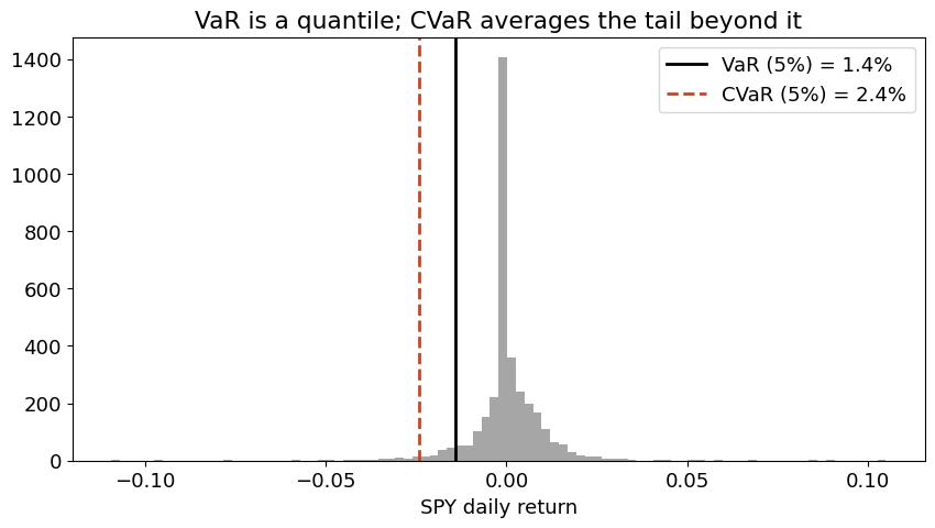
The Value-at-Risk (VaR) is simply a quantile of the distribution.

The \(\tau\)-day, \(\quant\) quantile VaR of an asset or portfolio is defined as \(\pnlVaRqtau\) such that

\[\Pr\left(\pnl_{t,t+\tau} \le \pnlVaRqtau_t\right) = \quant\]

where \(\pnl\) is the dollar amount of the pnl

\[\pnl = \port_{t+\tau}-\port_t\]

and \(\port\) is the value of the portfolio.

This says that…

there is a probability of \(\quant\)
that over a horizon of \(\tau\) days
the portfolio PnL will be less than\(\pnlVaRqtau\).

\[\Pr\left(\loss_{t,t+\tau} > L^{\VaRqtau}\right) = \quant\]

Returns#

It is often useful to discuss the \(\VaR\) return, \(\rVaRqtau\):

\[\Pr\left(r_{t,t+\tau} \le \rVaRqtau_t\right) = \quant\]

Note that

\[\pnlVaRqtau_t = \rVaRqtau_t\, \port_t\]

Profits versus Losses#

Our definitions above imply that \(\pnlVaRqtau\) and \(\rVaRqtau\) will be negative numbers (for all interesting cases.)

Be careful to note that the \(\VaR\) may be defined with respect to

Left tail of profit, \(\pnl\)
Right tail of losses, (a positive number,) \(\loss = -\pnl\)

Below, the notation will focus on returns and PnL.

However, when discussing VaR, we will often focus on the absolute value.
This is a reason that some references will focus on losses, \(L\), to get a positive value for VaR.

Distribution#

If \(\pnl\) has a cumulative density function (cdf) that is

continuous
strictly increasing then we can simply write:

\[\pnlVaRqtau = \cdf_{\pnl}^{-1}(\quant)\]

where \(\cdf_{\pnl}\) denotes the (unspecified) cdf of returns, and \(\cdf^{-1}_{\pnl}\) is its inverse.

Similarly, we have

\[\rVaRqtau = \cdf_r^{-1}(\quant)\]

Technical Note#

If the distribution of returns (profits) does not have such a cdf, then we need a more general definition,

\[\pnlVaRqtau = \sup\left\{\pnl\; |\; \cdf_{\pnl}(\pnl)\le \quant\right\}\]

Similarly for returns, \(\rVaRqtau\).

r = rets['SPY'].dropna()
q = np.quantile(r, QUANTILE)
CVaR = -r[r <= q].mean()

fig, ax = plt.subplots()
ax.hist(r, bins=90, color='gray', alpha=0.7)
ax.axvline(q, color='black', lw=2, label=f'VaR (5%) = {-q:.1%}')
ax.axvline(r[r <= q].mean(), color='#b64c33', lw=2, ls='--', label=f'CVaR (5%) = {CVaR:.1%}')
ax.set_xlabel('SPY daily return')
ax.set_title('VaR is a quantile; CVaR averages the tail beyond it')
ax.legend()
plt.show()

../_images/dee72e625b6e856cc81080093d7d538946f97b17adceaf99f2d3496fe2709344.png

Normal Distribution#

\(\VaR\) will often be modeled using a normal distribution.

This may seem strange given the evidence we saw yesterday that returns are not normally distributed–especially for the tails!
Serious risk management would not rely on a normal distribution in most cases.
But the normal \(\VaR\) formulas are–if nothing else–an important way to quote and compare \(\VaR\).

Suppose that profits and returns are normally distributed. Focusing on returns,

\[r_{t,t+\tau} \sim \mathcal{N}\left(\mu_\tau,\sigma_\tau^2\right)\]

where the subscript \(\tau\) is a reminder that the mean and variance depend on the return horizon, \(\tau\).

Normal Formula#

Then from the results above, we immediately have

\[\rVaRqtau = \mu_\tau + \zscore_\quant\sigma_\tau\]

where \(\zscore_\quant\) is the value (z-score) of the standard normal cdf associated with quantile \(q\). That is, if \(\cdfz\) denotes the standard normal cdf, then

\[\cdfz(\zscore_\quant)=\quant\]

Note that this formula for \(\rVaRqtau\) immediately gives us \(\pnlVaRqtau\), recalling that

\[\pnlVaRqtau_t = \rVaRqtau_t\, \port_t\]

rows = {}
for a in ['SPY', 'HYG', 'USO', 'BTC']:
    x = rets[a].dropna()
    rows[a] = {'VaR 5% (emp)':  -np.quantile(x, 0.05),
               'VaR 5% (norm)': -(x.mean() + norm.ppf(0.05)*x.std()),
               'VaR 1% (emp)':  -np.quantile(x, 0.01),
               'VaR 1% (norm)': -(x.mean() + norm.ppf(0.01)*x.std())}
pd.DataFrame(rows).T.style.format('{:.1%}').set_caption(
    'At 5% the normal is close; at 1% it underestimates the fat left tail (USO, BTC)')

At 5% the normal is close; at 1% it underestimates the fat left tail (USO, BTC)
	VaR 5% (emp)	VaR 5% (norm)	VaR 1% (emp)	VaR 1% (norm)
SPY	1.4%	1.5%	3.0%	2.2%
HYG	0.6%	0.7%	1.2%	1.0%
USO	3.0%	3.3%	5.9%	4.7%
BTC	5.3%	5.7%	10.0%	8.1%

Lognormal#

Suppose that prices are lognormal, so that log returns are normal with a one-period mean of \(\mu\) and one-period variance of \(\sigma^2\).

Then we have the following formula for the \(\tau\) horizon,

\[\rlog_{t,t+\tau} \sim \mathcal{N}\left(\tau\mu,\tau\sigma^2\right)\]

If we additionally assume

log returns are iid
log return mean, \(\mu\) is zero.

then we get the result that \(\rlog^{\VaR}\) scales with the square root of the horizon:

\[\rlog^{\VaRqtau} = \sqrt{\tau}\rlog^{\VaR_{q,1}}\]

Punchline#

This formula is widely used as a convention, even though…

returns are not iid! (And typically the modeling within VaR will recognize that.)
mean is not zero
we typically use returns, not log returns!

Thus, for any \(\VaR\), (profits, returns, log returns,) you’ll typically see

\(\VaR\) compounding with the square root of the horizon.

Technical Point#

We could use log returns, but it would require a different formula for \(\VaR\) profits, and these would no longer be normally distributed.

\[\pnlVaRqtau = \port_t\left[\exp\left\{\tau\mu + \zscore_q\sqrt{\sigma}\right\}-1\right]\]

Conditional Value-at-Risk (CVaR)#

Definition#

Conditional VaR (CVaR), also widely known as Expected Shortfall (ES) is the expected value conditional on being less than the \(\VaR\) threshold.

\[\pnlCVaRqtau = \E\left[\pnl_{t,t+\tau}\, |\, \pnl_{t,t+\tau} < \pnlVaRqtau\right]\]

\[\rCVaRqtau = \E\left[r_{t,t+\tau}\, |\, r_{t,t+\tau} < \rVaRqtau\right]\]

\[\pnlCVaRqtau_t = \rCVaRqtau_t \port_t\]

Normal Distribution#

Suppose we continue with the normal distribution of returns from above.

The \(\CVaR\) is the conditional expectation of a normal distribution, which gives us the following:

\[\rCVaRqtau_t =\; \mu_{\tau,t} - \frac{\pdfz(\zscore_\quant)}{\quant}\sigma_{\tau,t}\]

Technical Point#

We get the closed-form solution for \(\CVaR\) from an well-known result about the truncated normal distribution. That is to say, the conditional expectation of a normal distribution.

Consider a standard normal, \(\zscore\)
Let \(\pdfz\) denote the pdf of the standard normal.

It is well known that for any threshold, \(a\),

\[\E\left[\zscore\, |\, \zscore < a\right] = -\frac{\pdfz(a)}{\cdfz(a)}\]

Sufficient Statistics of a Normal#

Note the similarity between the formulas for \(\VaR\) and \(\CVaR\) when assuming a normal distribution:

\[\rVaRqtau = \mu_{\tau,t} + \underbrace{\zscore_\quant}\sigma_{\tau,t}\]

\[\rCVaRqtau = \mu_{\tau,t} + \underbrace{-\frac{\pdf_\zscore\left(\zscore_\quant\right)}{\quant}}\sigma_{\tau,t}\]

This is not a surprise.

The normal distribution is completely characterized by its mean and variance.
That is, these two parameters are sufficient statistics for a normal variable.
Any statistic of a normal distribution can be rewritten as a function of \(\mu\) and \(\sigma\).

Rescaled volatility#

Thus, \(\VaR\), \(\CVaR\), etc are all just rescalings of volatility if we are using a normal model.

In some sense, this is what normal \(\VaR\) is really about–having a scaled volatility.

Coherence#

Is \(\VaR\) a coherent risk measure?

No. In general, it is not subadditive.

Examples#

Payoffs#

Consider the payoff outcomes for \(\pnl_i\) and \(\pnl_j\) across 5 potential states of the world:

\[\begin{split}\pnl_i \in \begin{bmatrix}-2\\-1\\0\\1\\2\end{bmatrix}, \hspace{1cm} \pnl_j \in \begin{bmatrix}-1\\-2\\0\\1\\2\end{bmatrix}\end{split}\]

The states are ordered, such that in state \(s\), both securities deliver the payoff in row \(s\) of their respective arrays.

Consider a portfolio payoff that is the sum of the two: \(\pnl_p = \pnl_i + \pnl_j\).

What is

\[\pnl_i^{\VaR_{.2}}, \hspace{1cm} \pnl_j^{\VaR_{.2}}, \hspace{1cm} \pnl_i^{\VaR_{.2}} + \pnl_j^{\VaR_{.2}}, \hspace{1cm} \pnl_p^{\VaR_{.2}}\]

Example: Returns Not Subadditive#

Suppose there are 100 potential outcomes (“states”). We have two assets, \(r_i\) and \(r_j\).

In almost every state, the return is simply

\[r_{s,i} = r_{s,j} = \frac{s-50}{100}\]

The only exception is the two worst states, where the assets swap:

\[r_{i,(5)} = -.45, \quad r_{j,(5)} = -.46\]

\[r_{i,(4)} = -.46, \quad r_{j,(4)} = -.45\]

For each return individually,

\[r_i^{\VaR_{.05}} = -.45 = r_j^{\VaR_{.05}}\]

Yet for the equal-weighted portfolio, \(r_p = .5\, r_i + .5\, r_j\),

\[r_p^{\VaR_{.05}} = -.455\]

Data example#

On real, diversified assets VaR is almost always subadditive: pooling two return series lowers the quantile. The failure is a knife-edge that needs discrete tail events - options, credit - whose worst outcomes land on different days. Across every pair of our ETFs, it never fails:

from itertools import combinations
def var(x): return -np.quantile(x.dropna(), QUANTILE)

pairs = list(combinations(rets.columns.drop('SHV'), 2))
viol = sum(var(rets[[a,b]].dropna().mean(axis=1)) > (var(rets[a]) + var(rets[b]))/2 + 1e-9
           for a, b in pairs)
print(f'{viol} of {len(pairs)} ETF pairs violate VaR subadditivity')

0 of 45 ETF pairs violate VaR subadditivity

Normal VaR#

Is Normal VaR coherent?

CVaR#

Is CVaR coherent?

For a normal distribution?
For the examples above?

Value at Risk (VaR)

Contents

Value at Risk (VaR)#

Definition#

Returns#

Profits versus Losses#

Distribution#

Technical Note#

Normal Distribution#

Normal Formula#

Lognormal#

Punchline#

Technical Point#

Conditional Value-at-Risk (CVaR)#

Definition#

Normal Distribution#

Technical Point#

Sufficient Statistics of a Normal#

Rescaled volatility#

Coherence#

Examples#

Payoffs#

Example: Returns Not Subadditive#

Data example#

Normal VaR#

CVaR#