Contextual Alertness

Contextual Alertness#

Project Statement#

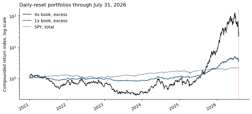
At the December 31, 2024 close a fictional long-short equity fund, Contextual Alertness, holds six memory, optical-networking and data-center names against six application-software names: 400% gross, 0% net, equal weights within each sleeve. The book is a stylized stand-in inspired by a real fund’s publicly reported positioning. It is not that fund’s holdings. Over the next eighteen months the book rises many-fold, then loses most of that gain in four sessions, July 24 to 29, 2026.

You are the risk manager. Take the book as given. Measure its risk, locate where the risk sat, say what a one-day VaR could and could not have told you, and build the version of the same strategy you would have been willing to run.

Context#

Long, +1/3 of NAV each	Theme	Short, -1/3 of NAV each	Theme
`SNDK`	memory and storage	`ADBE`	application software
`MU`	memory	`CRM`	application software
`VRT`	data-center power and cooling	`ORCL`	enterprise software
`LITE`	optical networking	`NOW`	enterprise software
`COHR`	optical networking	`WDAY`	application software
`BE`	data-center power	`MDB`	database software

The long sleeve is +200% of NAV and the short sleeve -200%, so gross exposure is 400% and net exposure is zero. The SNDK column is one strategy slot: it carries WDC returns through February 21, 2025 and SNDK returns from February 24, 2025, when Sandisk began regular-way trading; the switch is already in the supplied series.

The fund runs a mandate. At every close the book is reset to the target weights, so gross stays at 4x and net at zero: the 4x book. Dividing every weight by four gives the 1x book, the same positions at 100% gross.

Everything through July 31, 2026 is yours to study. The holdout, August 3 to October 26, 2026, exists for one purpose: Section 6 has you declare criteria, build controls on the design window, then run them, unchanged, on the holdout. Do not tune anything to it. If you study it earlier, the test in 6.3 stops measuring anything.

Data#

File	Sheets	Frequency	Sample
`data/project_situational_awareness_20261026.xlsx`	`descriptions`, `total return indexes`, `total returns`, `baseline weights`, `data source`, `checks`	daily	2020-12-31 to 2026-10-26

The total returns sheet holds the twelve names, SPY, QQQ, SMH, the eleven sector ETFs (XLK XLI XLF XLC XLRE XLE XLY XLB XLV XLU XLP) and SHV, as gross-dividend total returns. descriptions gives each ticker’s name, theme and side; baseline weights gives the twelve target weights.

Notes#

Returns are daily, close to close, simple total returns. A weight set at the close of $t$ earns the return of $t+1$: $r^{\text{book}}_{t+1} = \boldsymbol{w}_t' \boldsymbol{r}_{t+1}$. Annualize with 252 trading days.
The daily reset is a strategy-index convention: resetting to the target weights at every close makes 4x the book’s exposure on every day, so Sections 3 to 5 measure the risk of a fixed-leverage book. Section 2 shows what the convention assumes away.
Cash is SHV. Names and factors enter every regression in excess of SHV. The book’s weights sum to zero, so its return $\boldsymbol{w}'\boldsymbol{r}$ is already an excess return and its Sharpe ratio uses it directly; the fund’s NAV earns SHV on top of it.
VaR and CVaR are positive loss magnitudes, one-day at the 5% level unless a question says otherwise. A forecast for day $t$ uses data through $t-1$. A breach is a day whose realized loss exceeds the VaR forecast made for it. EWMA uses $\lambda = 0.94$ and a zero mean; you choose how to initialize $\sigma^2$ and state it.
The design window ends July 31, 2026. The report window is January 2, 2025 to July 31, 2026. The holdout runs from August 3, 2026 to October 26, 2026, the end of the file. Use the design window for all estimation and design. Open the holdout once, in 6.3, to evaluate the controls and criteria already specified. The final recommendation in 7.4 may use that verdict; do not re-tune the controls on the holdout.
The four-day loss is the compounded loss of the daily-reset 4x book over July 24 to 29, 2026, $1 - \prod_{t=1}^{4}(1 + r_t)$, with $r_t$ the book’s daily return.
Ignore financing, stock-borrow fees, transaction costs, taxes and market impact.

Data Preview#

from pathlib import Path
import numpy as np
import pandas as pd
import matplotlib.pyplot as plt

DATA = Path('../data/project_situational_awareness_20261026.xlsx')
descriptions = pd.read_excel(DATA, sheet_name='descriptions').set_index('ticker')
returns = pd.read_excel(DATA, sheet_name='total returns', index_col='Date', parse_dates=True)
weights = pd.read_excel(DATA, sheet_name='baseline weights').set_index('ticker')['equal-sleeve weight']

DESIGN_END = pd.Timestamp('2026-07-31')
print(f'{returns.shape[1]} series, {returns.index[0].date()} to {returns.index[-1].date()}; design window ends {DESIGN_END.date()}')

27 series, 2021-01-04 to 2026-10-26; design window ends 2026-07-31

design_returns = returns.loc[:DESIGN_END]
assert design_returns.index.max() <= DESIGN_END
book_4x = design_returns[weights.index] @ weights
book_1x = book_4x / 4
nav = pd.DataFrame({'4x book, excess': (1 + book_4x).cumprod(), '1x book, excess': (1 + book_1x).cumprod(), 'SPY, total': (1 + design_returns['SPY']).cumprod()})

fig, ax = plt.subplots(figsize=(10, 4.5))
nav.plot(ax=ax, color=['#14181e', '#1f4e79', '#8a8f98'], lw=1.2)
ax.axvspan(pd.Timestamp('2026-07-24'), DESIGN_END, color='#c1121f', alpha=0.10)
ax.set_yscale('log'); ax.set_ylabel('Compounded return index, log scale'); ax.set_xlabel('')
ax.set_title('Daily-reset portfolios through July 31, 2026', loc='left')
ax.legend(frameon=False); ax.spines[['top', 'right']].set_visible(False)
plt.show()

reversal = returns[['SPY', 'SMH', 'XLK', 'SHV']].loc['2026-07-20':'2026-07-31']
reversal.index = reversal.index.strftime('%Y-%m-%d')
reversal.style.format('{:+.2%}', na_rep='-').set_caption('Factor returns around the reversal')

../_images/954fa702b524437439d4fbb229ed6572a69c790c9064c693eef6bb192a97cc10.png

Factor returns around the reversal
	SPY	SMH	XLK	SHV
Date
2026-07-20	-0.16%	+0.41%	+0.07%	+0.01%
2026-07-21	+0.83%	+4.52%	+2.89%	-0.01%
2026-07-22	-0.12%	+0.48%	-0.28%	+0.02%
2026-07-23	-1.23%	-1.15%	-1.01%	-0.01%
2026-07-24	+0.10%	-3.27%	-1.44%	+0.03%
2026-07-27	+0.02%	-2.25%	-0.90%	+0.01%
2026-07-28	+0.24%	-3.45%	-1.84%	+0.03%
2026-07-29	-1.54%	-4.79%	-2.64%	+0.03%
2026-07-30	+1.68%	+6.88%	+5.50%	+0.01%
2026-07-31	+0.72%	+0.30%	-0.22%	+0.03%

1. The Book as Given#

1.1#

Verify the long, short, gross and net exposures as multiples of NAV and as dollars on $100 million of NAV. Then, for the 4x book and the 1x book, report over 2021-01-04 to 2026-06-30 and over 2025-01-02 to 2026-06-30:

annualized mean and volatility, Sharpe ratio, skewness, excess kurtosis
worst day, empirical 5% VaR and CVaR
maximum drawdown with its peak and trough dates, and cumulative return

Group the statistics by how they respond to leverage. Explain the scaling and compounding within each group.

1.2#

Report the compounded calendar-year return of the 4x book for 2021 through 2026 (to July 31), with the contribution of each sleeve, defined as the sum of the sleeve’s daily weighted returns. The sleeve contributions add to the sum of the book’s daily returns rather than to its compounded year; report both. In which years did the short sleeve add to the return, and in which did it subtract?

1.3#

Over both windows in 1.1, report

the average pairwise correlation among the long names, among the short names, and between a long and a short name
the correlation between the long basket’s return and the short basket’s return

What, if anything, does the short sleeve hedge?

1.4#

For each window in 1.1, report the standard error of the 4x book’s annualized mean and of its Sharpe ratio, and the Sharpe ratio’s 95% band. You are reviewing the book on June 30, 2026 with the statistics from 1.1 to 1.4 in hand. Which window would you base a risk assessment on, and what is a Sharpe ratio estimated on eighteen months of daily data evidence of? Answer in a short paragraph that uses the standard errors.

Estimation Error#

Under independence, the standard error of an annualized mean estimated from $N$ years of daily data is $\sigma_{\text{ann}}/\sqrt{N}$. With $q = 252$ periods a year, the annualized Sharpe ratio has standard error $\sqrt{(1 + \text{SR}^2/2q)/N}$.

2. The Reset#

2.1#

Start on 2025-01-02 with $100 million of NAV and positions set to the 4x target weights at the prior close. Hold cash as collateral without interest. Compare three rules:

Reset to target weights at every close.
Reset at every month-end close.
Hold the initial shares without rebalancing.

Gross exposure is measured at each close for the following day. Report:

NAV and gross leverage through July 31, 2026, as plots.
For each rule: gross exposure set on June 22 and July 23, NAV relative to its initial value on June 22, the July 24 to 29 return, and whether and when NAV reaches zero.
For fixed shares initialized on 2021-01-04: maximum gross exposure and minimum NAV, with their dates.
For fixed shares initialized at the July 23, 2026 close to the 4x target on $100 million: NAV, long exposure, short exposure, and gross leverage at each of the four closes through July 29. Compare NAV with the daily-reset portfolio over the same four days.

Could a fund have maintained each path? Use the gross exposures and NAV paths to explain what daily resetting assumes about the fund as a going concern, which convention a real fund lives under, and why the same positions lose different fractions of NAV over the reversal.

3. One-Day VaR Through the Reversal#

3.1#

Compute the EWMA volatility forecast of the 4x book from the first day your initialization allows to July 31, 2026, and, for every day in the design window, three one-day 5% VaR forecasts and the CVaR of each: historical simulation, Normal EWMA and filtered historical simulation.

Plot the EWMA forecast annualized; report the forecast made for July 24, 2026 and the fraction of forecasts for days through June 30, 2026 that were lower.
Report the three VaR and CVaR forecasts made at the July 23, 2026 close.

VaR Conventions#

Historical simulation: minus the 5% quantile of the trailing 252 daily returns; the CVaR is minus the mean of the returns at or below that quantile. Normal EWMA: $\text{VaR}_t = -z_{0.05}\,\sigma_t$ and $\text{CVaR}_t = \sigma_t\,\phi(z_{0.05})/0.05$, with $\sigma_t$ the EWMA forecast. Filtered historical simulation: standardize each past return by the EWMA forecast that applied to it, $z_s = r_s/\sigma_s$; take the 5% quantile and the tail mean of the standardized returns over the trailing 252 days, the same window as the historical simulation; multiply both by the current forecast $\sigma_t$.

3.2#

Backtest the three methods over 2025-01-02 to 2026-07-23 and over 2021-01-04 to 2024-12-31. For each method and window report

the number of forecasts, the number of breaches and the hit ratio
the longest run of consecutive breaches
the mean realized loss on breach days beside the mean CVaR forecast on those days

A method whose window has not yet filled starts later; report its count and say so. Which methods are calibrated in each window, and where the hit ratio is near 5%, does the breach-day loss match the CVaR forecast?

3.3#

For each of the four reversal days, July 24, 27, 28 and 29, report the realized loss of the 4x book as a multiple of the VaR each method had forecast for that day, and the four-day loss as a multiple of $\sqrt{4}$ times each method’s July 23 forecast.

Over 2025-01-02 to 2026-07-31, compare overlapping 4-day returns of the 4x book with $\sqrt{4}$ times the Normal EWMA one-day VaR in force at the start of each window. Report:

The hit ratio.
The largest ratio of realized loss to scaled VaR, with its date.

For each method, count the reversal-day breaches. Does the four-day loss challenge $\sqrt{h}$ scaling? Say which of its assumptions (independent daily returns, constant volatility, a zero mean) could account for the gap between the scaled forecast and the realized loss, and what one four-day realization can and cannot establish about them. Is the largest one-day ratio on a reversal day?

3.4#

Using the July 23 EWMA volatility scaled by $\sqrt{4}$ and a zero mean, compute the probability under the normal of a four-day loss at least as large as the one realized. Compute it again by drawing four standardized returns at random from the 252-day FHS window, re-inflating them by the July 23 volatility, and compounding. Then recompute the FHS VaR and CVaR forecasts made at the July 23 close, and this probability, with a 504-day standardization window.

Report the probabilities, and the 504-day VaR and CVaR beside the 252-day ones.
Report the worst standardized return in each window, its date, and whether one draw of it reaches the realized loss.

Say what that one observation does to the estimate, how far the conclusion depends on keeping it, and what each probability is a statement about: the model, the volatility level, or the book.

4. Where the Risk Sat#

Section 4 uses daily excess returns and two estimation windows: 2021-01-04 to 2024-12-31 and 2025-01-02 to 2026-06-30. The 1x book keeps the betas readable; multiply by four for the 4x book.

4.1#

Regress each of the twelve names, the long sleeve (+50% of NAV at 1x), the short sleeve (-50%) and the 1x book on two factor sets: SPY alone and SPY with SMH.

Report alpha, factor loadings, $R^2$ and residual volatility for the book and the two sleeves, annualized where appropriate. Use the individual-name regressions to verify the book’s exposure vector $B\boldsymbol{w}$; a full table of individual regressions is not required.

The book has zero net exposure. What is its market beta in each window, and which sleeve betas produce it? Did the short sleeve hedge the long sleeve’s largest exposure, add to it, or leave it alone?

Portfolio Exposures#

Regress each name’s excess return on the factor excess returns, $\tilde r_{i,t} = \alpha_i + \boldsymbol{\beta}_i' \tilde{\boldsymbol{f}}_t + \epsilon_{i,t}$, and stack the loadings in $B$, one column per name. The book with weights $\boldsymbol{w}$ has factor exposure $B\boldsymbol{w}$ and residual return $\boldsymbol{w}'\boldsymbol{\epsilon}_t$.

4.2#

Estimate the 1x book’s beta to SPY alone, and to SPY and SMH together, on a trailing one-year window at each quarter-end from September 2021 to June 2026. Tabulate or plot. The weights never changed. Did the exposures?

4.3#

For each factor set in 4.1 and each window, report the average pairwise correlation of the residuals among the long names, among the short names, and across the sleeves, next to the same averages for the raw returns. Then, for the 2025-01-02 to 2026-06-30 window, compute the 1x book’s variance three ways: from the sample covariance of the twelve names; from the factor model with a diagonal residual covariance; from the factor model with the full residual covariance. Do this for SPY alone and for SPY plus SMH.

Convert each variance to a 4x one-day Normal 5% VaR.

After the factors are removed, how many dimensions of risk are left in this book? Which term does the diagonal drop, and how large is it as a share of the book’s variance?

Variance Decomposition#

$\sigma^2_{\text{book}} = (B\boldsymbol{w})'\,\Sigma_f\,(B\boldsymbol{w}) + \boldsymbol{w}'\,\Sigma_\epsilon\,\boldsymbol{w}$. A factor risk model usually replaces $\Sigma_\epsilon$ with its diagonal; the sample covariance of the twelve names needs no such assumption.

4.4#

Attribute the July 24 to 29 loss of the 4x book to its factor exposure and its residual, as sums of daily contributions, using betas from each window and both factor sets from 4.1.

Report the systematic share under each of the four combinations.

Was the reversal a factor event or a residual event, and does the answer depend on what you call a factor?

5. Horizon and Survival#

5.1#

Compute daily log excess returns of the 1x and 4x books. For 2021-01-04 to 2024-12-31, 2025-01-02 to 2026-06-30 and 2021-01-04 to 2026-06-30, report

the annualized arithmetic mean, the annualized log mean, the annualized volatility, and the gap between the two means
for leverage 1x, 2x, 3x and 4x, the probability of underperforming cash over one month, one year and five years with the Barnstable formula, $\Pr\big[\texttt{r}_{t,t+h} < \texttt{r}^f_{t,t+h}\big] = \Phi\!\left(-\sqrt{h}\,\mu/\sigma\right)$, with $\mu$ and $\sigma$ the daily mean and standard deviation of the log excess return over cash
a plot of the probability against horizon for the four leverage levels on the 2021 to 2024 parameters

What sign does the 4x log mean take in each window, and what produces the gap? At each leverage, does a longer horizon raise or lower the probability? State in one sentence how this relates to the argument Barnstable’s trustees made about stocks.

Log Returns#

Write $\texttt{r}_t = \ln(1+r_t)$ for the log return.

5.2#

Simulate the probability that the 4x book suffers a maximum drawdown of at least 50% within one year and within five years, using the 2021-01-04 to 2026-06-30 parameters: once from a normal with the book’s daily log mean and standard deviation, once by resampling the book’s own daily returns. State the number of paths and random seed.

Compare the probabilities. Does the shape of the return distribution or the level of its volatility drive the answer? Explain how a drawdown from a running peak differs from a loss relative to initial wealth.

For each simulated path, cumulate log returns from initial wealth of one, track the running maximum including that initial value, and record the largest drawdown.

5.3#

As of June 30, 2026, what gross exposure would you have recommended for this mandate, on what criterion, and estimated on which window? Give the number and the reasoning.

6. The Risk-Managed Mandate#

The managed book keeps the twelve names, stays long the long sleeve and short the short sleeve, and never exceeds 4x gross. Every control uses only information available at the close before it acts. Every control is a rebalancing rule, and the constant-leverage comparators in 6.2 are daily-reset books at lower gross, so the comparison isolates timing from level.

6.1#

Before computing any Section 6 result, and before using any return after July 31, 2026, write a dated markdown cell that states

two numeric pass-fail criteria, one about risk and one about return or the cost of control
the control or controls you will test, chosen from a volatility target, a VaR or CVaR limit, a drawdown rule, a factor hedge, a sleeve or position cap, or a combination
every parameter

One well-motivated control is sufficient. You may use the risk measure or hedge developed in Section 7 as part of it; those questions still require their own analysis. Keep the original declaration. Record any revision in a second dated cell.

6.2#

Implement the declared controls on the design window. Over the report window, 2025-01-02 to 2026-07-31, for the managed book, the unmanaged 4x book, the 1x book, and a constant-leverage comparator whose gross exposure equals the managed book’s average gross over the report window, report

gross exposure through time and the dates on which the controls bound
cumulative return to July 23, the July 24 to 29 return, and cumulative return to July 31
annualized volatility, Sharpe ratio and maximum drawdown
average gross exposure, and the gross exposure set at the July 23 close (for July 24)

Compare each control with constant exposure at the same average gross leverage to distinguish timing from position size. State what each control cost or earned before the reversal and during it, against the unmanaged book and against its comparator, and whether an investor reviewing the managed book in April 2026 would have kept it.

6.3#

Run the same controls, unchanged, from August 3, 2026 to the end of the file, with the same comparators.

Report the same statistics plus the worst day.
Apply the criteria declared in 6.1: pass or fail, by your own test.

If the design window and the holdout disagree about a control, say which you believe and why.

7. Reporting and Recommendation#

Choose the additional risk measure, hedge specification, dashboard item, and final recommendation. Support each choice with the relevant comparison; the required analysis can justify different decisions.

7.1#

Propose one risk number a risk manager should have reported beside the one-day 5% VaR for this book, built from the same inputs. Define it, compute it daily through the design window, and report the forecast made at the June 22, July 1 and July 23, 2026 closes (for the following day). Justify the choice in course terms.

7.2#

Design a hedge overlay for the 4x book using trailing-window betas to one or more of SPY, SMH and the sector ETFs, refreshed at a frequency you choose.

Report the overlay positions as multiples of NAV.
Report the hedged book’s annualized volatility, Sharpe ratio and July 24 to 29 return over the report window, against the unhedged book.

Recommend for or against running it. Include the position sizes in the recommendation.

7.3#

Build the one-page view a risk manager should have had at the July 23, 2026 close, from data through that date only: a small table or a few figures covering

the volatility level and its history
the VaR and CVaR forecast made at that close (for the following day)
the drawdown from peak, the factor exposures, and one item of your choice

Produce the same page for the June 22, 2026 close. For each date, say in three or four sentences what the page showed and what action it supported.

7.4#

In half a page, state the gross exposure and controls under which you would run this mandate going forward, drawing on the design results and the holdout verdict in 6.3, what the mandate’s investors give up for them, and one observable result over the next year that would make you reverse the decision.

Deliverables#

Follow the Project Guidelines.