Long-Horizon Prediction with Persistent Signals

Data. CRSP value-weighted U.S. market index — monthly total returns, the dividend–price ratio (dividend yield), and the risk-free rate — from ../data/crsp_market_data.xlsx, monthly, 1926–2024. (Sheets: returns with columns crsp, sp500, rf, and metrics with dp_ratio_crsp, dp_ratio_sp500; this notebook uses the CRSP market series.) Source: CRSP via WRDS.

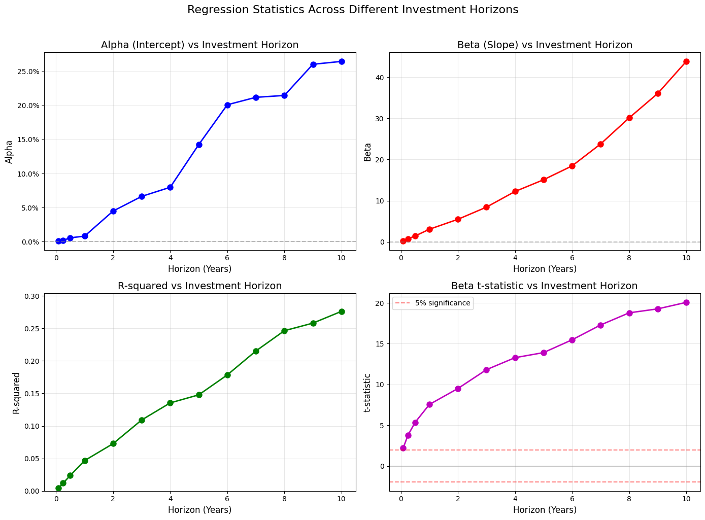
This notebook is the empirical companion to the forecasting slides. There we saw that the market’s dividend-price ratio (\(\text{DP}_t = D_t/P_t\)) barely forecasts next month’s return, yet predicts cumulative returns more and more strongly as the horizon lengthens.

Here we reproduce that pattern on CRSP value-weighted market data and trace it to a single cause: the dividend-price ratio is a highly persistent signal (an AR(1) coefficient near one), so its predictive content only accumulates into something visible over long horizons.

import pandas as pd
import numpy as np
import matplotlib.pyplot as plt

SHEET_RETS = 'returns'
SHEET_METRICS = 'metrics'
rets = pd.read_excel("../data/crsp_market_data.xlsx", sheet_name=SHEET_RETS, index_col=0, parse_dates=True)
metrics = pd.read_excel("../data/crsp_market_data.xlsx", sheet_name=SHEET_METRICS, index_col=0, parse_dates=True)

# This chapter uses the CRSP value-weighted market index (monthly, 1926-2024) and its
# dividend-price ratio. The data file also carries the S&P 500 (`sp500`, `dp_ratio_sp500`)
# and the risk-free rate (`rf`) if you want to extend the analysis.
rets = rets.rename(columns={"crsp": "rets"})
metrics = metrics.rename(columns={"dp_ratio_crsp": "dp ratio"})

HORZ = 5  # number of years; change this to desired horizon
FREQ = 12  # number of months per year

months = HORZ * FREQ

KEY_RETS = f'{HORZ}-year rets'
KEY_METRICS = 'dp annual'

data = pd.concat([rets['rets'], metrics['dp ratio']], axis=1)
data['dp annual'] = data['dp ratio'].rolling(window=FREQ).sum()
data['rets t+H'] = data['rets'].rolling(window=months).apply(lambda x: (x + 1).prod() - 1, raw=False)

#data['dp lag'] = data['dp smooth'].shift(months)
data[KEY_RETS] = data['rets t+H'].shift(-months)

import matplotlib.pyplot as plt
from matplotlib.ticker import FuncFormatter

fig, ax1 = plt.subplots(figsize=(10, 6))

label_fontsize = 16
tick_fontsize = 14
title_fontsize = 20

percent_formatter = FuncFormatter(lambda x, pos: '{:.0f}%'.format(x * 100))

color1 = 'tab:blue'
ax1.set_xlabel('Date', fontsize=label_fontsize)
ax1.set_ylabel(KEY_RETS, color=color1, fontsize=label_fontsize)
ax1.plot(data.index, data[KEY_RETS], color=color1, label=KEY_RETS)
ax1.tick_params(axis='y', labelcolor=color1, labelsize=tick_fontsize)
ax1.tick_params(axis='x', labelsize=tick_fontsize)
ax1.yaxis.set_major_formatter(percent_formatter)

ax2 = ax1.twinx()
color2 = 'tab:red'
ax2.set_ylabel(KEY_METRICS, color=color2, fontsize=label_fontsize)
ax2.plot(data.index, data[KEY_METRICS], color=color2, label=KEY_METRICS)
ax2.tick_params(axis='y', labelcolor=color2, labelsize=tick_fontsize)
ax2.yaxis.set_major_formatter(percent_formatter)

fig.tight_layout()
plt.title(f'{HORZ}-year Returns and Dividend-Price Ratio', fontsize=title_fontsize)
plt.show()

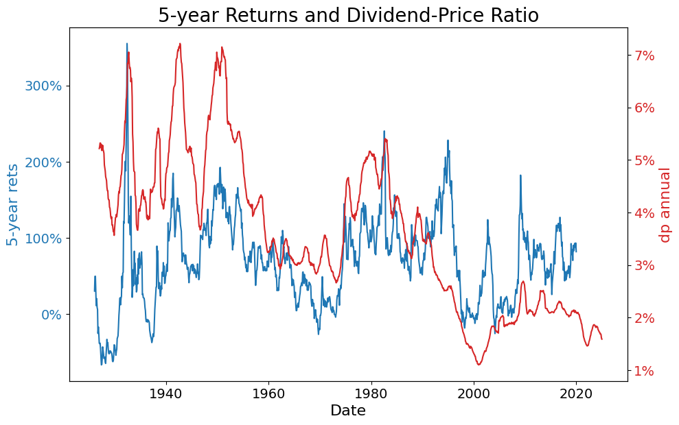
corr_rets_dp = data[KEY_RETS].corr(data[KEY_METRICS])
print(f'Correlation: {corr_rets_dp:.0%}')

Correlation: 38%

import statsmodels.api as sm
import pandas as pd
from IPython.display import display

# Remove NaN values for regression
reg_data = data[[KEY_RETS, KEY_METRICS]].dropna()

# Prepare data for regression
Y = reg_data[KEY_RETS]
X = reg_data[KEY_METRICS]

# Add constant to X for intercept
X_with_const = sm.add_constant(X)

# Run OLS regression
model = sm.OLS(Y, X_with_const)
results = model.fit()

# Extract key statistics
alpha = results.params['const']
beta = results.params[KEY_METRICS]
r_squared = results.rsquared
t_stat_beta = results.tvalues[KEY_METRICS]
p_value_beta = results.pvalues[KEY_METRICS]

# Prepare main summary dataframe (alpha, beta, r-squared)
summary_df = pd.DataFrame([
    [f"{alpha:.0%}", f"{beta:.1f}", f"{r_squared:.0%}"]
], columns=["alpha", "beta", "r-squared"], index=["OLS estimate"]).T

# Prepare t-stat and p-value dataframe for beta
beta_stats_df = pd.DataFrame(
    [ [f"{t_stat_beta:.1f}"], [f"{p_value_beta:.0%}"] ],
    columns=["beta"], 
    index=["t-stat", "p-value"]
)

display(summary_df)
display(beta_stats_df)

	OLS estimate
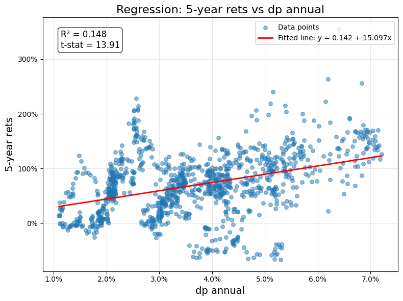
alpha	14%
beta	15.1
r-squared	15%

	beta
t-stat	13.9
p-value	0%

# Create scatter plot with regression line
fig, ax = plt.subplots(figsize=(8, 6))

# Scatter plot
ax.scatter(X, Y, alpha=0.5, s=30, label='Data points')

# Add regression line
X_plot = np.linspace(X.min(), X.max(), 100)
Y_pred = alpha + beta * X_plot
ax.plot(X_plot, Y_pred, 'r-', linewidth=2, label=f'Fitted line: y = {alpha:.3f} + {beta:.3f}x')

# Format axes
ax.set_xlabel(KEY_METRICS, fontsize=14)
ax.set_ylabel(KEY_RETS, fontsize=14)
ax.set_title(f'Regression: {KEY_RETS} vs {KEY_METRICS}', fontsize=16)

# Add grid
ax.grid(True, alpha=0.3)

# Format y-axis as percentage
ax.yaxis.set_major_formatter(FuncFormatter(lambda x, pos: '{:.0f}%'.format(x * 100)))
ax.xaxis.set_major_formatter(FuncFormatter(lambda x, pos: '{:.1f}%'.format(x * 100)))

# Add legend with regression statistics
legend_text = f'R² = {r_squared:.3f}\nt-stat = {t_stat_beta:.2f}'
ax.text(0.05, 0.95, legend_text, 
        transform=ax.transAxes, 
        fontsize=12,
        verticalalignment='top',
        bbox=dict(boxstyle='round', facecolor='white', alpha=0.8))

ax.legend(loc='upper right')
plt.tight_layout()
plt.show()

Various Horizons

import statsmodels.api as sm
import warnings
warnings.filterwarnings('ignore')

# Define the horizons to analyze (in years)
horizons = [1/12,.25,.5, 1, 2, 3, 4, 5, 6, 7, 8, 9, 10]

# Initialize dictionaries to store results
results_estimates = {}
results_tstats = {}
results_pvalues = {}

# Loop over each horizon
for HORZ in horizons:
    
    # Calculate the number of months
    months = round(HORZ * FREQ)
    
    # Prepare the data for this horizon
    data_temp = pd.concat([rets['rets'], metrics['dp ratio']], axis=1)
    data_temp['dp annual'] = data_temp['dp ratio'].rolling(window=FREQ).sum()
    data_temp['rets t+H'] = data_temp['rets'].rolling(window=months).apply(lambda x: (x + 1).prod() - 1, raw=False)
    data_temp[f'{HORZ}-year rets'] = data_temp['rets t+H'].shift(-months)
    
    # Set up regression variables
    key_rets_temp = f'{HORZ}-year rets'
    key_metrics_temp = 'dp annual'
    
    # Remove NaN values for regression
    reg_data = data_temp[[key_rets_temp, key_metrics_temp]].dropna()
    
    # Skip if not enough data
    if len(reg_data) < 30:  # Minimum observations for reasonable regression
        continue
    
    # Prepare data for regression
    Y = reg_data[key_rets_temp]
    X = reg_data[key_metrics_temp]
    
    # Add constant to X for intercept
    X_with_const = sm.add_constant(X)
    
    # Run OLS regression
    model = sm.OLS(Y, X_with_const)
    results = model.fit()
    
    # Store estimates
    results_estimates[HORZ] = {
        'Alpha': results.params['const'],
        'Beta': results.params[key_metrics_temp],
        'R-squared': results.rsquared,
        'N': len(reg_data)
    }
    
    # Store t-statistics
    results_tstats[HORZ] = {
        'Alpha t-stat': results.tvalues['const'],
        'Beta t-stat': results.tvalues[key_metrics_temp]
    }
    
    # Store p-values
    results_pvalues[HORZ] = {
        'Alpha p-value': results.pvalues['const'],
        'Beta p-value': results.pvalues[key_metrics_temp]
    }
    
    print(f"Completed horizon: {HORZ} years (N={len(reg_data)} observations)")

print("\nAll horizons processed successfully!")

Completed horizon: 0.08333333333333333 years (N=1176 observations)
Completed horizon: 0.25 years (N=1174 observations)
Completed horizon: 0.5 years (N=1171 observations)
Completed horizon: 1 years (N=1165 observations)
Completed horizon: 2 years (N=1153 observations)
Completed horizon: 3 years (N=1141 observations)

Completed horizon: 4 years (N=1129 observations)
Completed horizon: 5 years (N=1117 observations)
Completed horizon: 6 years (N=1105 observations)
Completed horizon: 7 years (N=1093 observations)
Completed horizon: 8 years (N=1081 observations)
Completed horizon: 9 years (N=1069 observations)
Completed horizon: 10 years (N=1057 observations)

All horizons processed successfully!

from IPython.display import display, HTML

# Create DataFrame for estimates
df_estimates = pd.DataFrame(results_estimates).T
df_estimates.index.name = 'Horizon (Years)'

# Create DataFrame combining t-stats and p-values
df_tstats = pd.DataFrame(results_tstats).T
df_pvalues = pd.DataFrame(results_pvalues).T

# Combine t-stats and p-values into one dataframe
df_stats = pd.DataFrame(index=df_tstats.index)
df_stats.index.name = 'Horizon (Years)'
df_stats['Alpha t-stat'] = df_tstats['Alpha t-stat']
df_stats['Alpha p-value'] = df_pvalues['Alpha p-value']
df_stats['Beta t-stat'] = df_tstats['Beta t-stat']
df_stats['Beta p-value'] = df_pvalues['Beta p-value']

# # Display DataFrame 1: Estimates
# display(HTML("<h3>Regression Estimates Across Horizons</h3>"))
# display(df_estimates.round(4))

# display(HTML("<h3>T-Statistics and P-Values Across Horizons</h3>"))
# display(df_stats.round(4))

# Create a summary DataFrame (raw values, no formatting/scaling)
summary_df = pd.DataFrame()
summary_df['Alpha'] = df_estimates['Alpha']
summary_df['Beta'] = df_estimates['Beta']
summary_df['R²'] = df_estimates['R-squared']
summary_df['Beta t-stat'] = df_stats['Beta t-stat']
summary_df['Significant?'] = df_stats['Beta p-value'] < 0.05  # 5% significance level
summary_df['N obs'] = df_estimates['N'].astype(int)

# Set index to formatted string (1 decimal) for horizon
summary_df.index = summary_df.index.map(lambda x: f"{x:.1f}")

# Display the summary DataFrame with formatting using .style
display(HTML("<h3>Summary: Dividend-Price Ratio Predictive Power Across Horizons</h3>"))
display(
    summary_df.style
        .format({
            'Alpha': '{:.1%}',
            'Beta': '{:.1f}',
            'R²': '{:.1%}',
            'Beta t-stat': '{:.1f}',
            'N obs': '{:d}'
        })
        .set_table_styles([{'selector': 'th', 'props': [('text-align', 'center')]}])
        .set_properties(subset=['Alpha','Beta','R²','Beta t-stat', 'Significant?','N obs'], **{'text-align': 'center'})
)

Summary: Dividend-Price Ratio Predictive Power Across Horizons

	Alpha	Beta	R²	Beta t-stat	Significant?	N obs
Horizon (Years)
0.1	0.1%	0.2	0.4%	2.2	True	1176
0.2	0.2%	0.7	1.2%	3.8	True	1174
0.5	0.6%	1.4	2.4%	5.3	True	1171
1.0	0.8%	3.1	4.7%	7.5	True	1165
2.0	4.5%	5.5	7.3%	9.5	True	1153
3.0	6.6%	8.4	10.9%	11.8	True	1141
4.0	8.0%	12.2	13.5%	13.3	True	1129
5.0	14.2%	15.1	14.8%	13.9	True	1117
6.0	20.1%	18.5	17.8%	15.5	True	1105
7.0	21.2%	23.8	21.5%	17.3	True	1093
8.0	21.5%	30.1	24.6%	18.8	True	1081
9.0	26.0%	36.0	25.8%	19.3	True	1069
10.0	26.5%	43.8	27.6%	20.1	True	1057

# Create visualizations of how regression statistics change with horizon
fig, axes = plt.subplots(2, 2, figsize=(14, 10))

# Plot 1: Alpha across horizons
ax1 = axes[0, 0]
ax1.plot(df_estimates.index, df_estimates['Alpha'], 'bo-', linewidth=2, markersize=8)
ax1.axhline(y=0, color='gray', linestyle='--', alpha=0.5)
ax1.set_xlabel('Horizon (Years)', fontsize=12)
ax1.set_ylabel('Alpha', fontsize=12)
ax1.set_title('Alpha (Intercept) vs Investment Horizon', fontsize=14)
ax1.grid(True, alpha=0.3)
ax1.yaxis.set_major_formatter(FuncFormatter(lambda x, pos: '{:.1f}%'.format(x * 100)))

# Plot 2: Beta across horizons
ax2 = axes[0, 1]
ax2.plot(df_estimates.index, df_estimates['Beta'], 'ro-', linewidth=2, markersize=8)
ax2.axhline(y=0, color='gray', linestyle='--', alpha=0.5)
ax2.set_xlabel('Horizon (Years)', fontsize=12)
ax2.set_ylabel('Beta', fontsize=12)
ax2.set_title('Beta (Slope) vs Investment Horizon', fontsize=14)
ax2.grid(True, alpha=0.3)

# Plot 3: R-squared across horizons
ax3 = axes[1, 0]
ax3.plot(df_estimates.index, df_estimates['R-squared'], 'go-', linewidth=2, markersize=8)
ax3.set_xlabel('Horizon (Years)', fontsize=12)
ax3.set_ylabel('R-squared', fontsize=12)
ax3.set_title('R-squared vs Investment Horizon', fontsize=14)
ax3.grid(True, alpha=0.3)
ax3.set_ylim([0, max(df_estimates['R-squared']) * 1.1])

# Plot 4: Beta t-statistics across horizons
ax4 = axes[1, 1]
ax4.plot(df_stats.index, df_stats['Beta t-stat'], 'mo-', linewidth=2, markersize=8)
ax4.axhline(y=1.96, color='red', linestyle='--', alpha=0.5, label='5% significance')
ax4.axhline(y=-1.96, color='red', linestyle='--', alpha=0.5)
ax4.axhline(y=0, color='gray', linestyle='-', alpha=0.3)
ax4.set_xlabel('Horizon (Years)', fontsize=12)
ax4.set_ylabel('t-statistic', fontsize=12)
ax4.set_title('Beta t-statistic vs Investment Horizon', fontsize=14)
ax4.grid(True, alpha=0.3)
ax4.legend()

plt.suptitle('Regression Statistics Across Different Investment Horizons', fontsize=16, y=1.02)
plt.tight_layout()
plt.show()

---

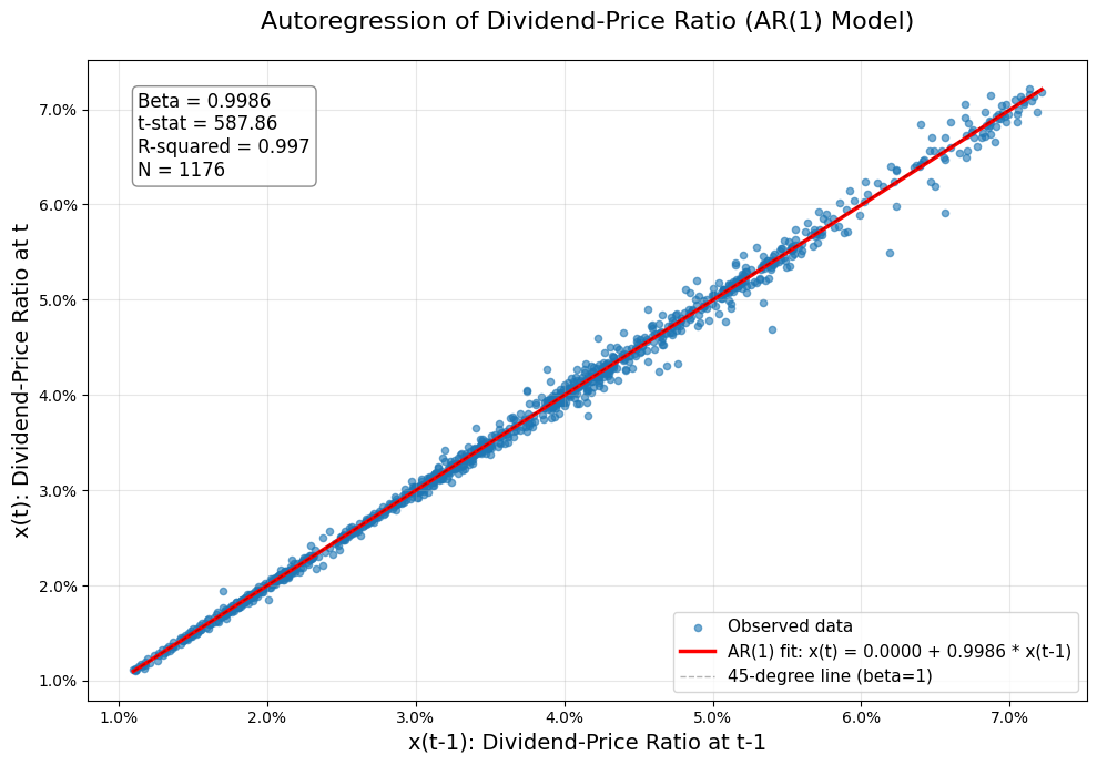
Autoregression of the Dividend-Price Ratio

Now we examine the persistence of the dividend-price ratio by running an autoregression (AR(1) model):

x(t) = alpha + beta × x(t-1) + error(t)

where x(t) is the dividend-price ratio at time t.

import statsmodels.api as sm
import pandas as pd
from IPython.display import display

# Prepare data for autoregression
ar_data = data[['dp annual']].dropna().copy()

# Create lagged variable (one-step ahead)
ar_data['dp annual lagged'] = ar_data['dp annual'].shift(1)

# Remove rows with NaN (from lagging)
ar_data = ar_data.dropna()

# Set up regression: x(t) = alpha + beta * x(t-1) + epsilon
Y = ar_data['dp annual']
X = ar_data['dp annual lagged']

# Add constant for intercept
X_with_const = sm.add_constant(X)

# Run OLS regression
ar_model = sm.OLS(Y, X_with_const)
ar_results = ar_model.fit()

# Extract key statistics
ar_alpha = ar_results.params['const']
ar_beta = ar_results.params['dp annual lagged']
ar_r_squared = ar_results.rsquared
ar_t_stat_alpha = ar_results.tvalues['const']
ar_t_stat_beta = ar_results.tvalues['dp annual lagged']
ar_p_value_alpha = ar_results.pvalues['const']
ar_p_value_beta = ar_results.pvalues['dp annual lagged']

# Create main results dataframe
ar_main_results = pd.DataFrame([
    [f"{ar_alpha:.6f}", f"{ar_beta:.6f}", f"{ar_r_squared:.4f}", len(ar_data)]
], columns=["Alpha", "Beta", "R-squared", "N"], index=["AR(1) Estimates"])

# Create t-statistics and p-values dataframe
ar_stats_results = pd.DataFrame([
    [f"{ar_t_stat_alpha:.3f}", f"{ar_t_stat_beta:.3f}"],
    [f"{ar_p_value_alpha:.4f}", f"{ar_p_value_beta:.4f}"]
], columns=["Alpha", "Beta"], index=["t-statistic", "p-value"])

# Display results
display(ar_main_results)
display(ar_stats_results)

	Alpha	Beta	R-squared	N
AR(1) Estimates	0.000020	0.998572	0.9966	1176

	Alpha	Beta
t-statistic	0.310	587.862
p-value	0.7565	0.0000

# Visualization of the autoregression
fig, ax = plt.subplots(figsize=(10, 7))

# Scatter plot
ax.scatter(X, Y, alpha=0.6, s=20, label='Observed data')

# Add regression line
X_plot = np.linspace(X.min(), X.max(), 100)
Y_pred = ar_alpha + ar_beta * X_plot
ax.plot(X_plot, Y_pred, 'r-', linewidth=2.5, label=f'AR(1) fit: x(t) = {ar_alpha:.4f} + {ar_beta:.4f} * x(t-1)')

# Add 45-degree line for reference (perfect persistence would be beta=1)
min_val = min(X.min(), Y.min())
max_val = max(X.max(), Y.max())
ax.plot([min_val, max_val], [min_val, max_val], 'k--', alpha=0.3, linewidth=1, label='45-degree line (beta=1)')

# Format axes
ax.set_xlabel('x(t-1): Dividend-Price Ratio at t-1', fontsize=14)
ax.set_ylabel('x(t): Dividend-Price Ratio at t', fontsize=14)
ax.set_title('Autoregression of Dividend-Price Ratio (AR(1) Model)', fontsize=16, pad=20)

# Format axes as percentage
ax.yaxis.set_major_formatter(FuncFormatter(lambda x, pos: '{:.1f}%'.format(x * 100)))
ax.xaxis.set_major_formatter(FuncFormatter(lambda x, pos: '{:.1f}%'.format(x * 100)))

# Add grid
ax.grid(True, alpha=0.3)

# Add statistics box
stats_text = f'Beta = {ar_beta:.4f}\nt-stat = {ar_t_stat_beta:.2f}\nR-squared = {ar_r_squared:.3f}\nN = {len(ar_data)}'
ax.text(0.05, 0.95, stats_text, 
        transform=ax.transAxes, 
        fontsize=12,
        verticalalignment='top',
        bbox=dict(boxstyle='round', facecolor='white', edgecolor='gray', alpha=0.9))

ax.legend(loc='lower right', fontsize=11)
plt.tight_layout()
plt.show()