


Betting Against Beta#
Project Statement#
In HW4 the cross-sectional regression of mean excess returns on market betas, across the 25 size-value portfolios, came out flatter than the CAPM predicts: a positive intercept and a slope below the market premium. Read as a trade, a flat line says that low-beta stocks earn more per unit of beta than high-beta stocks. A book long low-beta stocks levered up and short high-beta stocks levered down, to zero market beta, would then collect a premium while hedged to the market.
You have a panel of every US common stock since 1963. Estimate betas with the information available at the time, reproduce the line on your own sorts, build the book, change one construction choice and defend it, measure the book’s risk and cost, and tell an allocator whether to run it.
Context#
Homework 4 supplied portfolio betas. Here, estimate each stock’s beta at month-end using trailing monthly returns. Sorting on estimated betas can concentrate positive estimation errors in the high-beta group and negative errors in the low-beta group. Compare the estimates used to form portfolios with their subsequently realized betas.
The strategy scales each leg to an estimated market beta of one, taking the low-beta leg long and the high-beta leg short. Errors in the estimates affect both portfolio membership and leverage.
Data#
File |
What it holds |
Sample |
|---|---|---|
|
Return, price, shares, market cap, volume, exchange and share codes, delisting code and flag for every common stock on NYSE, AMEX and Nasdaq |
1963-01 to 2026-09 |
|
|
1963-01 to 2026-09 |
|
Ticker and company name history by |
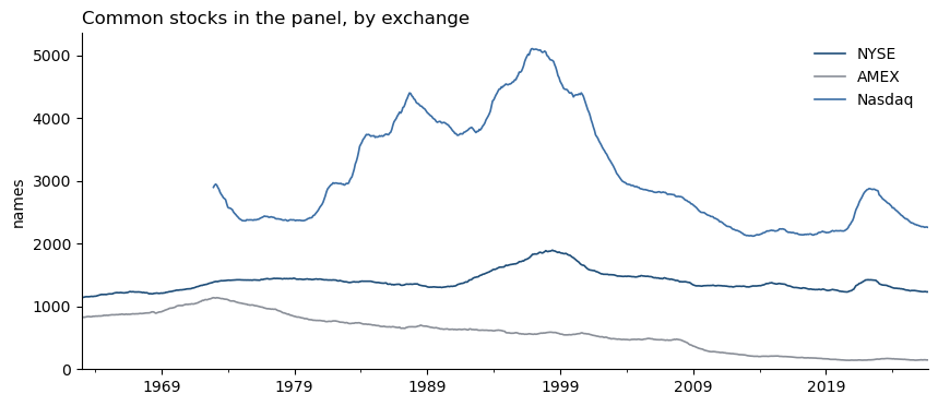
The supplied sample ends in September 2026. All references to the end of the data mean that date; the period from 2014 contains twelve years and nine months. A permno identifies a security through name and ticker changes. The panel contains ordinary common shares of US-incorporated companies on NYSE, AMEX and Nasdaq (exchcd 1, 2 or 3). Stocks enter and leave as their classifications change; delisting months are retained. There is no survivorship screen. Nasdaq enters in December 1972.
Returns include dividends. A stock’s delisting return is compounded into its last month, and the column dl_adj says how: 0 untouched, 1 CRSP’s own delisting return, 2 a replacement value for a performance delisting with no CRSP return (-30% on NYSE and AMEX, -55% on Nasdaq). The supplied returns already include this adjustment. State that you used the adjusted returns. A missing ret means CRSP had no valid return that month. No price, size or liquidity screen has been applied. Monthly vol is in shares; mktcap is in millions of dollars.
Notes#
Monthly simple returns. A portfolio formed at month end \(t\) uses only data through \(t\) and earns the return of month \(t+1\). Weights for month \(t+1\) use the market cap at \(t\).
Excess returns are returns minus
RF. The market isMkt-RF. Annualize means by 12 and volatilities by \(\sqrt{12}\); Sharpe ratios use excess returns.Alpha and beta of a return series are the intercept and slope of an OLS regression on
Mkt-RF. Report the alpha annualized with its plain OLS t-statistic, as in HW4; the same convention applies to every t-statistic in this brief.Set membership, ranks and weights at \(t\) using the stocks in the panel with a beta estimate, positive market cap and a price at \(t\), excluding stocks already marked as delisted (
dlstcdpresent). Apply any additional screen at that date. Keep the supplied delisting-adjusted returns.For a held stock whose return in \(t+1\) is missing, carry its value unchanged for that month: total return zero, excess return \(-R_{f,t+1}\). Keep its formation weight; do not remove it or reweight the other stocks. This is a valuation convention for missing observations. Omit missing returns when estimating betas.
The first 60-month betas, at their 36-month minimum, are available at the end of 1965, so every full-sample exhibit runs from 1966-01 to the end of the data. Say so in your tables.
The long-short book’s return is a self-financing excess return. Report its drawdown on the compounded path of that excess return, and say so.
Ignore transaction costs, financing and stock-borrow fees except where a question supplies them.
Data Preview#
from pathlib import Path
import numpy as np
import pandas as pd
import matplotlib.pyplot as plt

DATA = Path('data')                                  # the folder holding the parquet files
MONTHLY_FILE, FACTOR_FILE = 'crsp_monthly_1963_2026.parquet', 'ff_factors_monthly.parquet'
monthly = pd.read_parquet(DATA / MONTHLY_FILE)
ff = pd.read_parquet(DATA / FACTOR_FILE)
print(f'{len(monthly):,} stock-months, {monthly.permno.nunique():,} permnos, {monthly.date.min().date()} to {monthly.date.max().date()}')
sample = monthly[monthly.permno == 14593].tail(3).set_index('date')[['ret', 'prc', 'mktcap', 'vol', 'dl_adj']]
sample.index = sample.index.strftime('%Y-%m')
sample = sample.rename(columns={'ret': 'Return', 'prc': 'Price, $', 'mktcap': 'Market cap, $m', 'vol': 'Volume, shares', 'dl_adj': 'Delisting flag'})
display(sample.style.format({'Return': '{:+.2%}', 'Price, $': '{:.2f}', 'Market cap, $m': '{:,.0f}', 'Volume, shares': '{:,.0f}', 'Delisting flag': '{:.0f}'}, na_rep='—').set_caption('Example security: permno 14593, last three months'))
factor_preview = ff[['Mkt-RF', 'RF']].tail(3).rename(columns={'Mkt-RF': 'Market excess return', 'RF': 'Bill return'})
factor_preview.index = factor_preview.index.strftime('%Y-%m')
display(factor_preview.style.format({c: '{:+.2%}' for c in factor_preview.columns}, na_rep='—').set_caption('Monthly factor returns'))

ret = monthly.pivot(index='date', columns='permno', values='ret')       # one column per permno
cap = monthly.pivot(index='date', columns='permno', values='mktcap')
ex = ret.sub(ff['RF'].reindex(ret.index), axis=0)                      # excess returns, aligned to the factor file
print(f'wide panel: {ret.shape[0]} months by {ret.shape[1]:,} permnos')
3,518,948 stock-months, 26,519 permnos, 1963-01-31 to 2026-09-30
| Return | Price, $ | Market cap, $m | Volume, shares | Delisting flag | |
|---|---|---|---|---|---|
| date | |||||
| 2026-07 | +6.76% | 308.91 | 4,508,288 | 1,180,382,562 | 0 |
| 2026-08 | +2.66% | 316.85 | 4,624,166 | 895,574,132 | 0 |
| 2026-09 | +5.10% | 333.02 | 4,860,154 | 889,821,703 | 0 |
| Market excess return | Bill return | |
|---|---|---|
| date | ||
| 2026-07 | -0.61% | +0.33% |
| 2026-08 | +2.56% | +0.29% |
| 2026-09 | -1.07% | +0.31% |
wide panel: 765 months by 26,519 permnos
names = monthly.groupby(['date', 'exchcd']).size().unstack('exchcd').rename(columns={1: 'NYSE', 2: 'AMEX', 3: 'Nasdaq'})
fig, ax = plt.subplots(figsize=(10, 4))
names.plot(ax=ax, color=['#1f4e79', '#8a8f98', '#3b6ea5'], lw=1.2)
ax.set_title('Common stocks in the panel, by exchange', loc='left'); ax.set_ylabel('names'); ax.set_xlabel(''); ax.set_ylim(bottom=0)
ax.legend(frameon=False); ax.spines[['top', 'right']].set_visible(False)
plt.show()

dl = monthly.groupby('dl_adj').size().rename('stock-months').to_frame()
dl['share'] = dl['stock-months'] / dl['stock-months'].sum()
dl.index = ['0: untouched', '1: CRSP delisting return compounded in', '2: replacement value compounded in']
display(dl.style.format({'stock-months': '{:,.0f}', 'share': '{:.2%}'}, na_rep='-').set_caption('The delisting flag'))
| stock-months | share | |
|---|---|---|
| 0: untouched | 3,496,364 | 99.36% |
| 1: CRSP delisting return compounded in | 20,176 | 0.57% |
| 2: replacement value compounded in | 2,408 | 0.07% |
1. Betas With Information Available at the Time#
1.1#
For every stock and every month end, estimate the trailing 60-month beta on monthly excess returns, requiring at least 36 months with a return.
At each December from 1973 to the last December in the data, report the number of stocks in the panel at that date with an estimate, and the 10th, 50th and 90th percentiles of those estimates. One table or one figure.
Note#
At month end \(t\), regress stock \(i\)’s monthly excess return on the market’s over the trailing \(W\) months in which the stock has a return:
Under independence the standard error of \(\hat\beta_{i,t}\) is about \(\sigma_\varepsilon / (\sigma_m \sqrt{W})\), so a stock whose residual volatility is twice the market’s carries a standard error near 0.26 on sixty months. A beta dated \(t\) is used with the return of month \(t+1\).
1.2#
At each month end from 1965-12, rank the stocks with an estimate on the beta dated that month, form ten equal-count groups by rank (a stock at a breakpoint goes to the lower group), and hold each group for the following month, value-weighted by market cap at the formation date. For each decile over 1966-01 to the end of the data, report
the average pre-ranking beta and the post-ranking beta
the annualized mean excess return, the alpha with its t-statistic, the Treynor ratio and the information ratio
a plot of mean excess return against post-ranking beta, with the CAPM line through the origin at the sample market premium and the fitted line with an intercept
Note#
The pre-ranking beta of a group is the weighted average, with the portfolio’s weights, of the stock-level estimates that put the stocks there. The post-ranking beta is the slope of the group’s realized return on the market over the holding months. The line is drawn against the post-ranking beta.
1.3#
Estimate a second beta for every stock and month end from the trailing 36 months, requiring at least 24. For holding months from 1966-01 to the end of the data, report
the Spearman rank correlation across stocks between the 36-month and the 60-month estimates, averaged over formation dates
the share of the stocks below the median on the 60-month estimate that are also below the median on the 36-month estimate
forming deciles on each estimator over the same holding months, the slope of post-ranking on pre-ranking decile betas for each estimator
What does the difference between the two windows say about measurement error in beta? The default book in Section 3 uses the 60-month estimate; say whether your evidence argues for a different window, and why.
2. What the Returns Say About the CAPM#
Use the deciles from 1.2 over 1966-01 to the end of the data unless a question says otherwise.
2.1#
Regress the deciles’ mean excess returns on their post-ranking betas, with an intercept.
Report the intercept and the slope with t-statistics, the \(R^2\), and the sample market premium beside the slope.
Repeat with the pre-ranking betas as the regressor.
2.2#
Compute the joint statistic \(H\) on the ten alphas and its p-value. Then repeat 2.1 and this question on 1966-01 to 2013-12 and on 2014-01 to the end of the data.
Note#
With \(\boldsymbol{\hat\alpha}\) the \(n\) alphas, \(\hat\Sigma_\epsilon\) the covariance of the \(n\) residual series and \(\text{SR}_m\) the market’s monthly Sharpe ratio over the same months (the mean of its monthly excess return over the standard deviation of that return, not annualized),
under the null that all alphas are zero.
2.3#
Regress the post-ranking decile betas on the pre-ranking decile betas over the full sample and report the slope. Re-form the deciles on the convex combination \(\beta^*\) with that slope as the weight \(w\).
Report which numbers in 2.1 and 2.2 change and which do not, and say why.
This is a statement about the sort, made in sample; a weight used to size positions in Section 4 must come from data before the months it is applied to.
Note#
Write the estimate as \(\hat\beta_i = \beta_i + e_i\). If the error is independent of the true beta, a regression of post-ranking decile betas on pre-ranking decile betas has slope \(\text{var}(\beta)/(\text{var}(\beta)+\text{var}(e))\), and a cross-sectional regression on pre-ranking betas is attenuated toward zero by the same factor. The convex combination \(\beta^*_{i,t} = w\,\hat\beta_{i,t} + (1-w)\) pulls every estimate toward one.
2.4#
In half a page, compare the CAPM’s predictions for the table and plot in 1.2 with your evidence. Address the intercept, the slope relative to the premium, the joint test and its sub-period results, and measurement error. What does the evidence support, and what can this sample not establish?
3. The Default Book#
The construction is fixed so that every group’s Section 4 starts from the same book.
Betas: trailing 60 months, at least 36, on monthly excess returns, combined with one at \(w = 0.6\). The weight is a convention fixed by the brief, so that every group’s default is the same book; it is not derived from 2.3, and 2.3 does not identify it.
Legs: at each month end, the stocks in the panel with a beta, positive market cap and a price are ranked on the combined beta and split at the median rank. The lower half is the long leg and the upper half the short leg; with an odd count, the middle stock goes to the long leg.
Weights within each leg: rank weights.
Leverage: each leg is scaled to an ex-ante beta of one by its weighted average combined beta.
Cash: the remainder, at the bill rate.
Holding period one month, from 1966-01 to the end of the data.
If a construction loses more than its capital in a month, report the failure date and leverage. Exclude it from ordinary performance comparisons.
Note#
A portfolio with excess return \(\tilde r_L\) and beta \(\beta_L\), held in size \(L = 1/\beta_L\) per dollar of capital, has beta one. Holding \(L\) dollars of it means borrowing \(L-1\) at the bill rate, or holding \(1-L\) in bills if \(L<1\); the position’s excess return is \(L\,\tilde r_L\). The book pairs a long low-beta leg with a short high-beta leg, each scaled to beta one:
Its ex-ante beta is \(1 - 1 = 0\). The dollar position is \(1/\beta_L\) long and \(1/\beta_H\) short, and the cash position, \(1 - 1/\beta_L + 1/\beta_H\), earns the bill rate. The betas in the leverage are estimates dated \(t\); the beta the book turns out to have is the slope of \(\tilde r_{\text{book}}\) on the market.
Weights within a leg are set at the formation date and sum to one within the leg:
rule |
weight of stock \(i\) |
|---|---|
value |
proportional to its market cap at \(t\) |
equal |
\(1/N\) |
rank |
proportional to \(\lvert z_i - \bar z \rvert\), where \(z_i\) is the stock’s rank on beta within the whole cross section and \(\bar z\) the average rank; the stocks farthest from the median carry the most weight |
A leg’s ex-ante beta is the weighted average of its stocks’ betas with the same weights. Half the names in this panel sit below the NYSE 20th percentile of market cap, so the three rules describe different portfolios.
3.1#
Build the book. For each month record the two legs’ ex-ante betas, their leverages, the cash position and the number of stocks in each leg.
Report the median, minimum and maximum of each leverage and of the cash position.
Plot the long leg’s leverage through time.
3.2#
Report, for the book and for each leg unlevered
annualized mean excess return, volatility, Sharpe ratio with its standard error, skewness and worst month
maximum drawdown with its peak and trough dates
alpha with its t-statistic, and the realized beta from a regression on the market
Estimation Error#
Under independence, an annualized Sharpe ratio estimated from \(N\) years of data observed \(q\) times a year has standard error approximately \(\sqrt{(1 + \text{SR}^2/(2q))/N}\), with \(q = 12\) for monthly returns.
3.3#
Compare each leg’s average ex-ante beta with its realized beta. Explain the book’s realized beta from the two legs’ betas and the leverages applied to them. Three or four sentences.
3.4#
Report the book’s one-way turnover per month, and the share of each leg’s levered weight in stocks below the NYSE 20th percentile of market cap and in stocks priced under $5, averaged over the full sample and over 2014-01 to the end of the data.
Where does the composition say the book’s capacity would bind?
Turnover Convention#
One-way turnover per month is \(\sum_i \lvert w_{i,t} - w^{\text{drift}}_{i,t-1} \rvert\) over all names, with signed weights (positive in the long leg, negative in the short leg) that include the leg’s leverage: the sum of absolute changes across both legs, unhalved. The drifted weight is last month’s weight carried forward by the stock’s return and rescaled to last month’s gross exposure. The average starts with the second formation month; the first month is the initial purchase.
4. One Choice, Changed#
Choose one mechanism below and compare the baseline with at least one plausible alternative, holding the other elements fixed. Select an economically meaningful change and explain its effect. One well-developed investigation satisfies this section.
The beta estimate. The window; the weight on the estimate in the convex combination, including a weight of one or a weight estimated on an expanding window of past data; or how the leg’s beta that sets its leverage is measured.
Volatility against correlation. Beta is correlation times a ratio of volatilities. Sort on each component alone over the same trailing window and build the book on each sort, with the leverage still set by the combined beta.
Weights within the legs. Rank, value or equal.
Exclusions. A size screen, a price screen or a liquidity screen, stated as a rule applied at each formation date.
4.1#
Before computing, state the mechanism, the alternative or alternatives, exactly what stays fixed, and in one sentence what you expect to change.
4.2#
Build the alternative book or books. Report, side by side with the default
the table of 3.2, the leverage summary of 3.1, and the turnover and composition of 3.4
the Sharpe ratio with its standard error, the alpha with its t-statistic and the realized beta over 2014-01 to the end of the data
A construction that fails in the sense of Section 3 is reported as a failure and left out of the comparison.
4.3#
How did the change affect your conclusion about the baseline strategy? Identify the largest change in the reported results and explain it in course terms. Compare it with your expectation in 4.1.
5. Risk#
Run Sections 5 and 6 on the default book and on your Section 4 alternative.
5.1#
Before computing any result in Sections 5 and 6, write a dated markdown cell with two numeric pass-fail criteria an allocator would apply to this trade: one on the full sample and one on the period from 2014-01 or on implementation (cost, capacity or realized beta). Name the construction each criterion applies to. Keep the original declaration. Record any revision in a second dated cell.
5.2#
For each book, report its largest drawdown and one other episode that you choose as a useful contrast. Explain the choice. For both episodes report:
peak and trough dates, depth, recovery date or not recovered, and months under water counted from the peak
the market’s cumulative excess return from the peak to the trough
In which episodes did the book lose while the market gained, and what in the construction produces a loss of that kind? Two or three sentences.
Drawdown Dates#
Drawdown of a return path is its distance below its running maximum. The peak is the last month at the running maximum; months under water are counted from the peak to the month the path regains it.
5.3#
Report the rolling 36-month realized beta of each book as a plot, with its minimum and maximum and their dates, and the monthly 5% historical VaR and CVaR, the normal VaR, the skewness and the excess kurtosis.
5.4#
Estimate each book’s beta separately over the months in which the market excess return was positive and the months in which it was negative.
Report the two betas with t-statistics and the number of months in each group.
Say in one or two sentences what the pair adds to the single realized beta of 3.2.
6. Cost and Persistence#
6.1#
Apply the cost schedule below, using each name’s NYSE size quintile at the formation date. Report
the cost per year and the net Sharpe ratio under this schedule, over the full sample and over 2014-01 onward
the drag of a 50 basis point annual spread on a financing notional of \((L_L - 1)^+ + L_H\), the amount borrowed for the long leg plus the short proceeds
the break-even: the uniform one-way cost per unit traded, and the multiple of the high schedule, at which each book’s full-sample mean net return is zero
Say where the schedule sits relative to the break-even.
Trading Costs#
Assign each name to an NYSE size quintile at the formation date: compute the quintile breakpoints of market cap among NYSE names and place every name, whatever its exchange, by those breakpoints. A one-way cost per unit of traded weight applies by quintile, and the month’s cost is \(\sum_i \lvert w_{i,t} - w^{\text{drift}}_{i,t-1} \rvert \times c(q_i)\). The schedule is an illustrative assumption.
NYSE size quintile |
smallest |
2 |
3 |
4 |
largest |
|---|---|---|---|---|---|
high schedule |
100 bp |
50 bp |
30 bp |
20 bp |
10 bp |
6.2#
Report for each book over 1966-01 to 2013-12 and over 2014-01 to the end of the data
Sharpe ratio with its standard error, alpha with its t-statistic, and realized beta
the net Sharpe ratio under the high cost schedule
Using the standard errors, explain what the period since 2014 can establish about persistence and what it cannot. Compare its evidence with the longer pre-2014 window.
7. Recommendation#
7.1#
Apply the criteria declared in 5.1 to the default book and to your alternative. Report pass or fail for each construction. If the decisions differ, explain which construction you prefer and why.
7.2#
In at most half a page, recommend whether to invest. Specify the construction, universe, and leverage, and discuss capacity using 3.4 and 4.2. Use the persistence assessment in 6.2 and the other evidence to support the recommendation; identify what remains unresolved. A well-supported decision to reject the strategy is equally valid.
7.3#
State one observable result over the next \(N\) years that would reverse your recommendation. Choose \(N\) with the Sharpe standard-error formula and show the arithmetic.
Deliverables#
Follow the Project Guidelines.