VaR by Filtered Historical Simulation

The companion notebooks define VaR and model its volatility. Here we simulate the full one-day-ahead distribution of a portfolio, keeping the time-varying volatility, the cross-asset dependence, and the fat tails all at once.

The method:

• GARCH each asset for its volatility dynamics.

• Filter the returns by that volatility to get standardized shocks that are close to i.i.d.

• Bootstrap the shocks jointly (by date, so cross-asset dependence survives), re-inflate by the current volatility forecast, and rebuild the portfolio.

Sampling whole dates - not each asset on its own - is what preserves the covariance, with no separate correlation model.

import pandas as pd
import numpy as np
import matplotlib.pyplot as plt
%matplotlib inline
plt.rcParams['figure.figsize'] = (10,5)
plt.rcParams['font.size'] = 13

import warnings
warnings.filterwarnings("ignore")   # quiet arch convergence chatter
from arch import arch_model
from scipy.stats import norm

np.random.seed(2025)

LOADFILE = '../data/risk_etf_data.xlsx'
rets = pd.read_excel(LOADFILE, sheet_name='total returns').set_index('Date')

# a portfolio of the risky ETFs (drop the near-riskless bill fund)
assets = rets.columns.drop('SHV')
R = rets[assets].dropna()
w = np.full(len(assets), 1/len(assets))   # equal weight

FREQ = 252
QUANTILE = 0.05

The Portfolio

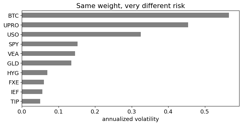
An equal-weight book across ten risky ETFs - one asset per major market. The weights are trivial; what matters is how differently these assets carry risk, from single-digit bond volatility to Bitcoin near 50%.

labels = {'SPY':'US equity', 'VEA':'Developed intl equity', 'UPRO':'US equity, 3x',
          'GLD':'Gold', 'USO':'Crude oil', 'FXE':'Euro FX', 'BTC':'Bitcoin',
          'HYG':'High-yield credit', 'IEF':'7-10y Treasury', 'TIP':'TIPS'}
holdings = pd.DataFrame({'asset class': [labels[a] for a in assets],
                         'weight': w,
                         'ann. vol': R.std().values*np.sqrt(FREQ)}, index=assets)
display(holdings.style.format({'weight':'{:.0%}','ann. vol':'{:.0%}'})
        .set_caption('Holdings'))

fig, ax = plt.subplots(figsize=(9,4))
(R.std()*np.sqrt(FREQ)).sort_values().plot.barh(ax=ax, color='gray')
ax.set_xlabel('annualized volatility')
ax.set_title('Same weight, very different risk')
plt.show()

Holdings

	asset class	weight	ann. vol
SPY	US equity	10%	15%
VEA	Developed intl equity	10%	15%
UPRO	US equity, 3x	10%	45%
GLD	Gold	10%	13%
USO	Crude oil	10%	32%
FXE	Euro FX	10%	6%
BTC	Bitcoin	10%	57%
HYG	High-yield credit	10%	7%
IEF	7-10y Treasury	10%	6%
TIP	TIPS	10%	5%

Volatility Dynamics

Fit a GARCH(1,1) to each asset. Keep two things per asset: the standardized residuals (return divided by its own conditional volatility - the shocks), and the one-step volatility forecast (today’s risk level).

Z  = pd.DataFrame(index=R.index, columns=assets, dtype=float)   # standardized shocks
CV = pd.DataFrame(index=R.index, columns=assets, dtype=float)   # conditional vol series
mu_fwd  = pd.Series(index=assets, dtype=float)                  # one-step mean forecast
sig_fwd = pd.Series(index=assets, dtype=float)                  # one-step vol forecast

for a in assets:
    res = arch_model(R[a]*100, mean='Constant', vol='GARCH', p=1, q=1).fit(disp='off')
    Z[a]  = res.std_resid
    CV[a] = res.conditional_volatility / 100
    fc = res.forecast(horizon=1, reindex=False)
    mu_fwd[a]  = fc.mean.iloc[-1, 0] / 100
    sig_fwd[a] = np.sqrt(fc.variance.iloc[-1, 0]) / 100

(sig_fwd*np.sqrt(FREQ)).sort_values(ascending=False).to_frame('ann. vol forecast').style.format('{:.1%}').set_caption('Current (one-step) volatility, annualized')

Current (one-step) volatility, annualized

	ann. vol forecast
UPRO	40.8%
BTC	39.2%
USO	34.0%
GLD	20.8%
VEA	16.5%
SPY	13.6%
FXE	4.7%
IEF	4.7%
TIP	4.2%
HYG	3.2%

Filtered Historical Simulation

Draw a historical date at random and take that day’s standardized shocks across all assets at once. Re-inflate each by its current volatility forecast, add the mean, and form the portfolio. Because we resample whole dates, the cross-asset dependence of the shocks carries through untouched.

Many draws give the one-day portfolio distribution; VaR and CVaR are its lower quantile and tail mean.

M = 50_000
Zv = Z.values
idx = np.random.randint(0, len(Zv), size=M)

asset_sim = mu_fwd.values + Zv[idx] * sig_fwd.values   # M x n, re-inflated to current vol
port_sim  = asset_sim @ w                               # M portfolio returns

cut = np.quantile(port_sim, QUANTILE)
VaR_fhs  = -cut
CVaR_fhs = -port_sim[port_sim <= cut].mean()
print(f'FHS  VaR(5%) = {VaR_fhs:.2%}    CVaR(5%) = {CVaR_fhs:.2%}')

FHS  VaR(5%) = 1.09%    CVaR(5%) = 1.73%

Comparison

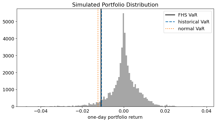
Against two unconditional benchmarks on the same portfolio: a normal fit and plain historical simulation.

At the latest date the three nearly agree - because current volatility happens to sit near its long-run average. That is not a coincidence to rely on: the next figure shows when they pull apart.

rp = R @ w
VaR_norm = -(rp.mean() + norm.ppf(QUANTILE)*rp.std())
VaR_hist = -np.quantile(rp, QUANTILE)

tab = pd.DataFrame({'VaR (5%)': [VaR_fhs, VaR_hist, VaR_norm]},
                   index=['Filtered historical (conditional)', 'Historical (unconditional)', 'Normal (unconditional)'])
display(tab.style.format('{:.2%}'))

fig, ax = plt.subplots()
ax.hist(port_sim, bins=120, color='gray', alpha=0.7)
ax.axvline(-VaR_fhs, color='black', lw=2, label='FHS VaR')
ax.axvline(-VaR_hist, color='C0', lw=2, ls='--', label='historical VaR')
ax.axvline(-VaR_norm, color='C1', lw=2, ls=':', label='normal VaR')
ax.set_xlabel('one-day portfolio return')
ax.set_title('Simulated Portfolio Distribution')
ax.legend()
plt.show()

	VaR (5%)
Filtered historical (conditional)	1.09%
Historical (unconditional)	1.08%
Normal (unconditional)	1.25%

VaR Through Time

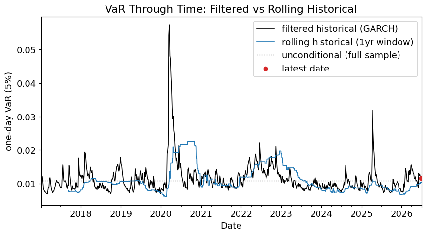
Re-evaluate the one-day VaR at every date, and compare like with like: a rolling historical VaR (a one-year window, recomputed daily) also conditions on the regime, so this is the fair benchmark.

The GARCH-filtered VaR reacts within days; the rolling window lags - a shock takes a year to enter the window and then lingers for a year before dropping out as a cliff. The full-sample line is only an anchor. At the latest date all three sit close, because current volatility is near its average.

mu_p = float(w @ R.mean().values)
Zw = Z.values                                  # T x n standardized shocks
rp  = pd.Series(R.values @ w, index=R.index)   # portfolio realized returns

WIN = 252                                      # one-year rolling window
roll_hist  = -rp.rolling(WIN).quantile(QUANTILE)   # conditional historical, recomputed daily
var_uncond = -rp.quantile(QUANTILE)            # full-sample anchor
dates = R.index[::5]                            # weekly, for a smooth FHS line
fhs_t = pd.Series([-(mu_p + np.quantile(Zw @ (w * CV.loc[t].values), QUANTILE)) for t in dates],
                  index=dates)

fig, ax = plt.subplots()
fhs_t.plot(ax=ax, color='black', lw=1.2, label='filtered historical (GARCH)')
roll_hist.plot(ax=ax, color='C0', lw=1.2, label='rolling historical (1yr window)')
ax.axhline(var_uncond, color='gray', ls=':', lw=1, label='unconditional (full sample)')
ax.scatter([fhs_t.index[-1]], [fhs_t.iloc[-1]], color='C3', zorder=5, label='latest date')
ax.set_ylabel('one-day VaR (5%)')
ax.set_title('VaR Through Time: Filtered vs Rolling Historical')
ax.legend()
plt.show()

VaR by Regime

One number summarizes the gap: historical VaR is fixed, while filtered VaR spans a wide range as the volatility regime moves.

summary = pd.Series({'calmest week':        fhs_t.min(),
                     'latest (calm now)':   fhs_t.iloc[-1],
                     'most stressed week':  fhs_t.max(),
                     'historical (fixed)':  var_uncond},
                    name='one-day VaR (5%)')
summary.to_frame().style.format('{:.2%}').set_caption('Filtered VaR moves; historical does not')

Filtered VaR moves; historical does not

	one-day VaR (5%)
calmest week	0.68%
latest (calm now)	1.16%
most stressed week	5.73%
historical (fixed)	1.08%

Backtesting: How Often Is VaR Breached?

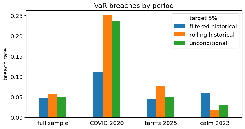
A 5% VaR should be breached about 5% of days - no more, and not bunched up. Compute each method’s one-day-ahead VaR at every date, then count the days the next return fell below it.

The full-sample rate is only half the story, and it flatters everyone. The breaches are not spread evenly: a method that ignores the regime over-breaches in stress, so by arithmetic it must under-breach elsewhere - over-conservative right after a crash (its window still carries it), then caught short by the next one. Split the count by period to see both halves: the crash of 2020, the tariff selloff of early 2025, and the calm of 2023 that still sat in the shadow of 2022.

rp = pd.Series(R.values @ w, index=R.index)          # daily portfolio return

# one-day-ahead VaR from each method, at every date
fhs_var    = pd.Series([-(mu_p + np.quantile(Zw @ (w*CV.iloc[i].values), QUANTILE)) for i in range(len(R))],
                       index=R.index)
roll_var   = -rp.rolling(252).quantile(QUANTILE)
uncond_var = pd.Series(-rp.quantile(QUANTILE), index=R.index)

methods = {'filtered historical': fhs_var, 'rolling historical': roll_var, 'unconditional': uncond_var}
periods = {'full sample':    slice(None),
           'COVID 2020':      slice('2020-02-19', '2020-04-30'),
           'tariffs 2025':    slice('2025-01-01', '2025-06-30'),
           'calm 2023':       slice('2023-01-01', '2023-12-31')}

def hit_rate(var, period):
    breach = (rp < -var.shift(1))[var.shift(1).notna()]
    return breach.loc[period].mean()

hits = pd.DataFrame({m: {p: hit_rate(v, sl) for p, sl in periods.items()} for m, v in methods.items()}).T
display(hits.style.format('{:.1%}').background_gradient(cmap='Reds', vmin=0.05, vmax=0.30)
        .set_caption('Share of days the next return breached the 5% VaR (target 5%)'))

ax = hits.T.plot.bar(figsize=(9,4.5), rot=0)
ax.axhline(0.05, color='black', ls='--', lw=1.2, label='target 5%')
ax.set_ylabel('breach rate'); ax.set_title('VaR breaches by period'); ax.legend()
plt.show()

Share of days the next return breached the 5% VaR (target 5%)

	full sample	COVID 2020	tariffs 2025	calm 2023
filtered historical	4.8%	11.1%	4.4%	6.0%
rolling historical	5.7%	25.0%	7.7%	1.9%
unconditional	5.0%	23.6%	5.0%	3.0%

Notes

• Why filtered. Dividing by the GARCH volatility removes the volatility clustering, leaving shocks that are close to i.i.d. Re-inflating by the current forecast makes the VaR respond to the regime.

• Why historical shocks. Bootstrapping the empirical residuals keeps the skew and fat tails that a normal draw would erase.

• Why sample whole dates. Resampling a date keeps every asset’s shock from the same day together, so the cross-asset dependence needs no separate correlation model.

• Scaling up. With a handful of assets we can fit a GARCH to each. For a large book (hundreds of names) you would first reduce to a few factors - e.g. sector portfolios - GARCH the factors, and handle the idiosyncratic piece separately. See LFD for Dimension Reduction for how much structure a few factors carry.