Market Timing

D/P is high. How much more of the market should you hold?

\[ w_t = \frac{f_t}{\gamma\,\sigma_t^2} \]

• \(f_t\): forecast of next month’s excess return, \(\tilde r_{t+1}\).

• \(\sigma_t^2\): conditional return variance; \(\gamma\): risk aversion.

• At a given variance, a higher return forecast means a larger market position.

• Horizon versus frequency: a longer-horizon forecast can still be updated when a new signal arrives. A persistent signal may imply similar positions across updates.

How Much to Tilt?

Write the linear forecast as

\[ f_t = \mu + R\sigma z_t \]

• \(\mu\), \(\sigma\): unconditional mean and volatility of excess returns.

• \(z_t\): signal standardized to mean zero and standard deviation one.

• \(R\): information coefficient (IC), the signal’s correlation with next month’s excess return.

• \(S=\mu/\sigma\): market Sharpe ratio. IC and Sharpe use the same monthly horizon and sample.

With known conditional moments and constant conditional variance,

\[ w_t = \bar w(1+\kappa z_t), \qquad \kappa=\frac{R}{S} \]

• Relative tilt: \(\kappa\) is the position change per signal standard deviation, divided by the average position \(\bar w\).

• Baseline matters: the same IC produces a larger proportional tilt when the market’s positive Sharpe ratio is lower.

• Higher Sharpe need not mean a smaller absolute response: hold IC, volatility, and risk aversion fixed. Doubling the expected return doubles the average position and halves \(\kappa\). The absolute position change is unchanged.

Campbell–Thompson: for small predictive \(R^2\), at fixed risk aversion,

\[ \text{Proportional expected-return gain} \approx \frac{R^2}{S^2}=\kappa^2 \]

• Here, \(R^2\) is the single-predictor regression’s in-sample \(R^2\), with an intercept.

• A small \(R^2\) can matter when the baseline Sharpe ratio is also small.

• This gain assumes known conditional moments. It excludes estimation error.

Show code

Hide code

crsp = pd.read_excel('../data/crsp_market_data.xlsx', sheet_name='returns', index_col='date', parse_dates=True)
metrics = pd.read_excel('../data/crsp_market_data.xlsx', sheet_name='metrics', index_col='date', parse_dates=True)
mkt = (crsp['crsp'] - crsp['rf']).rename('market')
dp = (metrics['dp_ratio_crsp'].rolling(12).sum() * 100).rename('D/P')
d = pd.concat([mkt.rename('y'), dp.shift(1).rename('x')], axis=1).dropna()
R, S = d['x'].corr(d['y']), d['y'].mean() / d['y'].std()
theory = pd.DataFrame([{'R²': R**2, 'IC': R, 'Monthly SR': S, 'κ': R / S,
                        'Expected-return gain': s_star(S, R**2)**2 / S**2 - 1}])
display(show(theory, {'R²': '{:.2%}', 'IC': '{:.3f}', 'Monthly SR': '{:.3f}', 'κ': '{:.2f}',
                     'Expected-return gain': '{:.0%}'},
             'CRSP market on lagged D/P, 1927–2026. Exact model-implied gain at fixed risk aversion.'))

CRSP market on lagged D/P, 1927–2026. Exact model-implied gain at fixed risk aversion.

R²	IC	Monthly SR	κ	Expected-return gain
0.40%	0.063	0.128	0.49	25%

• The 25% is a model-implied expected-return gain, not a 25% increase in Sharpe ratio.

Forecast Errors

• Returns: CRSP value-weighted market less the one-month Treasury; monthly, 1926–2026.

• Signal: D/P, the trailing 12-month sum of monthly income returns.

• Estimation: expanding OLS on lagged D/P; 20-year initial sample; forecasts from January 1947 through June 2026.

\[ R^2_{\mathrm{OOS}} = 1-\frac{\sum_t(\tilde r_{t+1}-f_t)^2} {\sum_t(\tilde r_{t+1}-\bar r_t)^2} \]

• Numerator: the forecasting regression’s squared errors.

• Denominator: squared errors from forecasting the expanding historical mean, \(\bar r_t\), known at the forecast date.

• Negative \(R^2_{\mathrm{OOS}}\): the regression forecasts worse than this naive benchmark.

• Forecast IC: correlation of \(f_t\) with \(\tilde r_{t+1}\) across forecast months. It can be negative and is not \(\sqrt{R^2_{\mathrm{OOS}}}\).

Show code

Hide code

market, ins_market = expanding_forecast(mkt, dp.to_frame(), 240)
forecast_fit = pd.DataFrame([{'Forecast IC': market['forecast'].corr(market['y']),
                              'R² OOS': oos_r2(market, market['forecast'])}])
display(show(forecast_fit, {'Forecast IC': '{:+.3f}', 'R² OOS': '{:.2%}'},
             'CRSP D/P forecast, 1947–2026. Positive correlation, larger squared errors than the historical mean.'))

CRSP D/P forecast, 1947–2026. Positive correlation, larger squared errors than the historical mean.

Forecast IC	R² OOS
+0.076	-0.58%

Correlation and Calibration

Suppose a forecast is always ten times the realized excess return:

\[ f_t = 10\tilde r_{t+1} \]

• IC = 1: perfect co-movement.

• Large errors: a 1% return was forecast as 10%; the error is 9 percentage points.

• Poor \(R^2_{\mathrm{OOS}}\): squared errors can exceed those of a naive forecast despite perfect correlation.

• Calibration: if the tenfold scale error is known, divide the forecast by ten.

• Position sizing: the original forecast produces ten times the position of the calibrated forecast under the same variance and risk aversion.

• Sharpe ratio: a constant positive rescaling changes leverage and risk but leaves Sharpe unchanged under this unconstrained linear rule.

• Feasible calibration: estimate it using information available before the next return. The forecast’s level and scale determine the position.

Reference: Empirical Results

Realized Performance

• Data: crsp_market_data.xlsx; the same CRSP/D/P sample used above.

• Both timing and historical-mean positions use the expanding variance of excess returns.

• The common risk-aversion scale is omitted; it does not affect Sharpe ratios.

• Floored D/P: set negative forecasts to zero, eliminating short market positions.

• ΔSR: realized Sharpe minus buy-and-hold Sharpe.

• SE of ΔSR: 2,000 paired bootstrap draws of months; both strategies use the same draws. This calculation does not preserve dependence across months.

Show code

Hide code

bh = market['y'].to_numpy()
benchmark_sr = sharpe(bh)
rows = [{'Strategy': 'Buy and hold', 'SR': benchmark_sr}]
for name, forecast in [('Historical mean', market['null']), ('D/P timing', market['forecast']),
                        ('D/P floored at zero', market['forecast'].clip(lower=0))]:
    strategy = (forecast / market['var'] * market['y']).to_numpy()
    row = {'Strategy': name, 'SR': sharpe(strategy), 'ΔSR': sharpe(strategy) - benchmark_sr,
           'SE of ΔSR': paired_se(strategy, bh)}
    if name != 'Historical mean':
        row.update({'R² OOS': oos_r2(market, forecast), 'IC': forecast.corr(market['y'])})
    rows.append(row)
results = pd.DataFrame(rows).set_index('Strategy')[['R² OOS', 'IC', 'SR', 'ΔSR', 'SE of ΔSR']]
display(show(results, {'R² OOS': '{:.2%}', 'IC': '{:+.3f}', 'SR': '{:.2f}',
                       'ΔSR': '{:+.3f}', 'SE of ΔSR': '{:.3f}'},
             'CRSP, 1947–2026. Annualized Sharpe ratios.'))

CRSP, 1947–2026. Annualized Sharpe ratios.

Strategy	R² OOS	IC	SR	ΔSR	SE of ΔSR
Buy and hold			0.54
Historical mean			0.51	-0.035	0.015
D/P timing	-0.58%	+0.076	0.45	-0.087	0.129
D/P floored at zero	-0.11%	+0.078	0.56	+0.014	0.108

• D/P timing underperforms buy-and-hold in this sample.

• Flooring raises the realized Sharpe to 0.56, versus 0.54 for buy-and-hold. The difference is small relative to its standard error.

When D/P Helped

• Top: D/P forecast and expanding historical mean; monthly forecasts multiplied by 12.

• Middle: D/P and its lowest value through 1990.

• Bottom: cumulative squared-error improvement, divided by the historical mean’s total squared error. Its endpoint is \(R^2_{\mathrm{OOS}}\).

Show code

Hide code

p = market
gain = ((p['y'] - p['null'])**2 - (p['y'] - p['forecast'])**2).cumsum() / ((p['y'] - p['null'])**2).sum()
low = dp.loc[:'1990'].min()
fig, (a1, a2, a3) = plt.subplots(3, 1, figsize=(9, 8.2), sharex=True, gridspec_kw={'height_ratios': [1.1, 0.9, 1]})
a1.plot(p.index, p['forecast'] * FREQ, color=NAVY, lw=1.4, label='D/P forecast')
a1.plot(p.index, p['null'] * FREQ, color=GREY, lw=1.4, ls='--', label='expanding historical mean')
a1.axhline(0, color=GREYL, lw=1)
a1.yaxis.set_major_formatter(PercentFormatter(1, decimals=0)); a1.set_ylabel('forecast, a year')
a1.set_title('Market excess return: out-of-sample forecasts, CRSP D/P')
a1.legend(loc='upper right', ncol=2, fontsize=10.5, handlelength=2.4); grid(a1)
d_oos = dp.loc[p.index[0]:]
a2.plot(d_oos.index, d_oos, color=INK, lw=1.4)
a2.axhline(low, color=GREY, lw=1, ls=':')
a2.annotate(f'lowest through 1990, {low:.2f}%', (d_oos.index[-1], low), xytext=(0, 4), textcoords='offset points', ha='right', fontsize=10, color=GREY)
a2.set_ylabel('D/P, %'); a2.set_title('Dividend-price ratio'); grid(a2)
a3.plot(gain.index, gain, color=INK, lw=1.4)
a3.axhline(0, color=GREYL, lw=1)
a3.axvspan(pd.Timestamp('1973-01-01'), pd.Timestamp('1975-12-31'), color=GREYL, alpha=0.5)
a3.annotate('1973-75', (pd.Timestamp('1974-06-30'), gain.loc['1975-12'].iloc[0]), xytext=(-60, 10), textcoords='offset points', fontsize=10)
pk = gain.idxmax(); cross = gain.loc[pk:][gain.loc[pk:] < 0].index[0]
a3.plot([pk], [gain.max()], 'o', color=NAVY, ms=5); a3.annotate(f'peak, {pk:%Y-%m}', (pk, gain.max()), xytext=(6, 4), textcoords='offset points', fontsize=10)
a3.plot([cross], [0], 'o', color=MAROON, ms=5)
a3.annotate(f'gain gone, {cross:%Y-%m}', (cross, 0), xytext=(28, 34), textcoords='offset points', fontsize=10,
            arrowprops=dict(arrowstyle='-', color=GREY, lw=0.8), bbox=dict(fc='white', ec='none', pad=1))
a3.yaxis.set_major_formatter(PercentFormatter(1, decimals=2))
a3.set_ylabel('cumulative R² gain'); a3.set_title('Rising: D/P beats the historical mean that month')
grid(a3); plt.tight_layout(); display(fig); plt.close(fig)

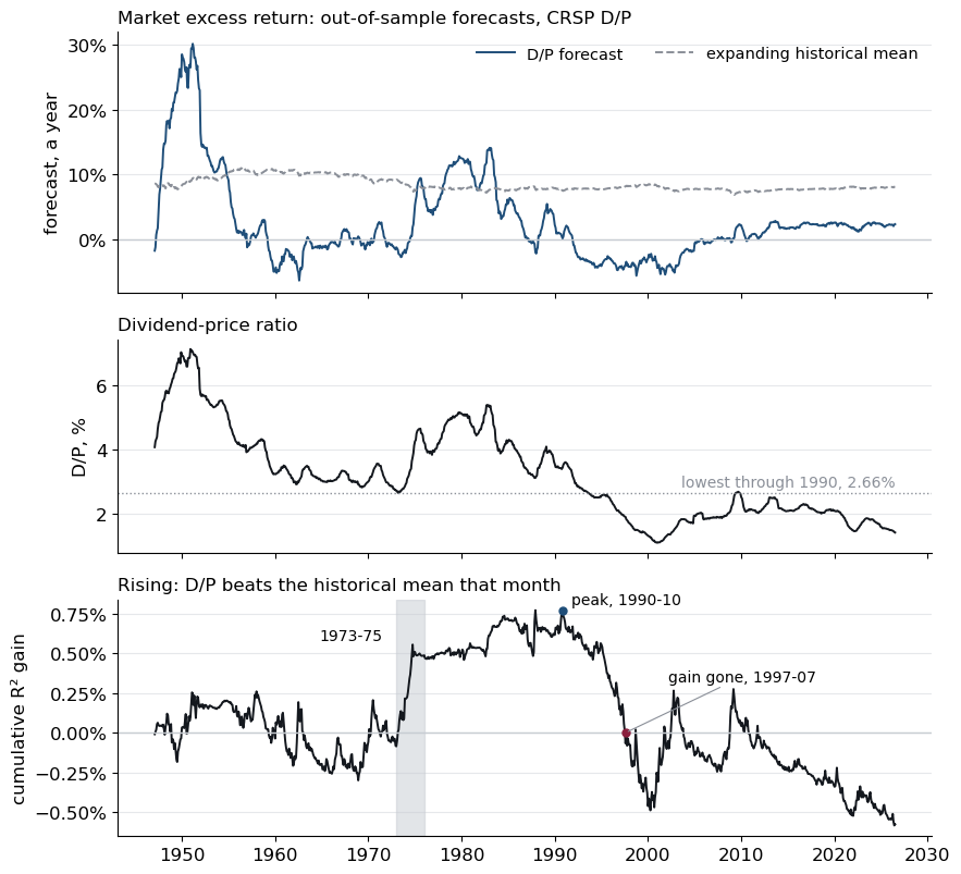
• Most of D/P’s forecasting advantage comes from 1973–75.

• From 1993, D/P falls below its pre-1991 low. The fitted line extrapolates to negative return forecasts and short market positions.

Forecast Level and Scale

• Forecast deviation: D/P forecast minus expanding historical mean.

• Timing bet: return on the position difference between these strategies.

• Information ratio (IR): the timing bet’s mean return divided by its volatility, annualized.

Show code

Hide code

dev = market['forecast'] - market['null']
diagnosis = pd.DataFrame({
    'Measure': ['Average forecast deviation', 'Average D/P position / average benchmark position',
                'Market excess return', 'Timing bet IR', 'Forecast-deviation SD',
                'Deviation-return correlation × return SD'],
    'Value': [f'{dev.mean() * FREQ:+.1%}',
              f"{(market['forecast'] / market['var']).mean() / (market['null'] / market['var']).mean():.2f}",
              f"{market['y'].mean() * FREQ:.1%}", f"{sharpe(dev / market['var'] * market['y']):.2f}",
              f'{dev.std() * FREQ:.1%}', f"{dev.corr(market['y']) * market['y'].std() * FREQ:.1%}"]
}).set_index('Measure')
display(show(diagnosis, {'Value': '{}'},
             'CRSP, 1947–2026. Return levels and forecast SDs: monthly × 12; IR annualized.'))

CRSP, 1947–2026. Return levels and forecast SDs: monthly × 12; IR annualized.

Measure	Value
Average forecast deviation	-5.7%
Average D/P position / average benchmark position	0.25
Market excess return	8.0%
Timing bet IR	-0.21
Forecast-deviation SD	6.7%
Deviation-return correlation × return SD	4.1%

• Level: forecasts were too low, leaving the strategy underinvested in a rising market.

• Scale: forecast deviations varied more than their correlation with returns supported.

• OLS benchmark: in sample, with an intercept, fitted-value volatility equals fitted-value/return correlation times return volatility.

• The fitted-value/return correlation is \(\sqrt{R^2}\). The raw signal’s correlation has the regression slope’s sign.

Model Details

The Campbell–Thompson calculation assumes the forecast is the true conditional mean, with constant residual variance:

\[ \sigma_\epsilon^2=(1-R^2)\sigma^2, \qquad \bar w=\frac{\mu}{\gamma\sigma_\epsilon^2}, \qquad \bar w\kappa=\frac{R\sigma}{\gamma\sigma_\epsilon^2} \]

• Absolute response: \(\bar w\kappa\) is the position change per signal standard deviation. It does not depend on \(\mu\).

• Lower volatility: holding positive expected return, positive IC, and risk aversion fixed, lower volatility raises Sharpe and reduces the relative tilt, while increasing the absolute response.

• Normalization: setting the average position to one gives \(w_t=1+\kappa z_t\). Maintaining that normalization as inputs change requires rescaling risk aversion.

The average squared conditional Sharpe ratio is

\[ S^{*2}=\frac{S^2+R^2}{1-R^2} \]

• Expected timing return: \(S^{*2}/\gamma\).

• Expected return on the constant position \(\mu/(\gamma\sigma^2)\): \(S^2/\gamma\).

• Exact proportional expected-return gain: \(S^{*2}/S^2-1\).

• \(S^{*2}\) averages conditional squared Sharpe ratios. It is not the realized strategy’s unconditional squared Sharpe ratio.

Sources

• Campbell and Thompson (2008), “Predicting Excess Stock Returns Out of Sample: Can Anything Beat the Historical Average?” Review of Financial Studies.

• Goyal and Welch (2008), “A Comprehensive Look at the Empirical Performance of Equity Premium Prediction.” Review of Financial Studies.