Comparing VaR Estimates

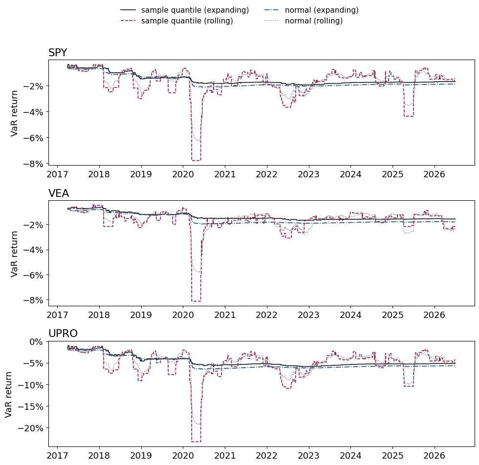
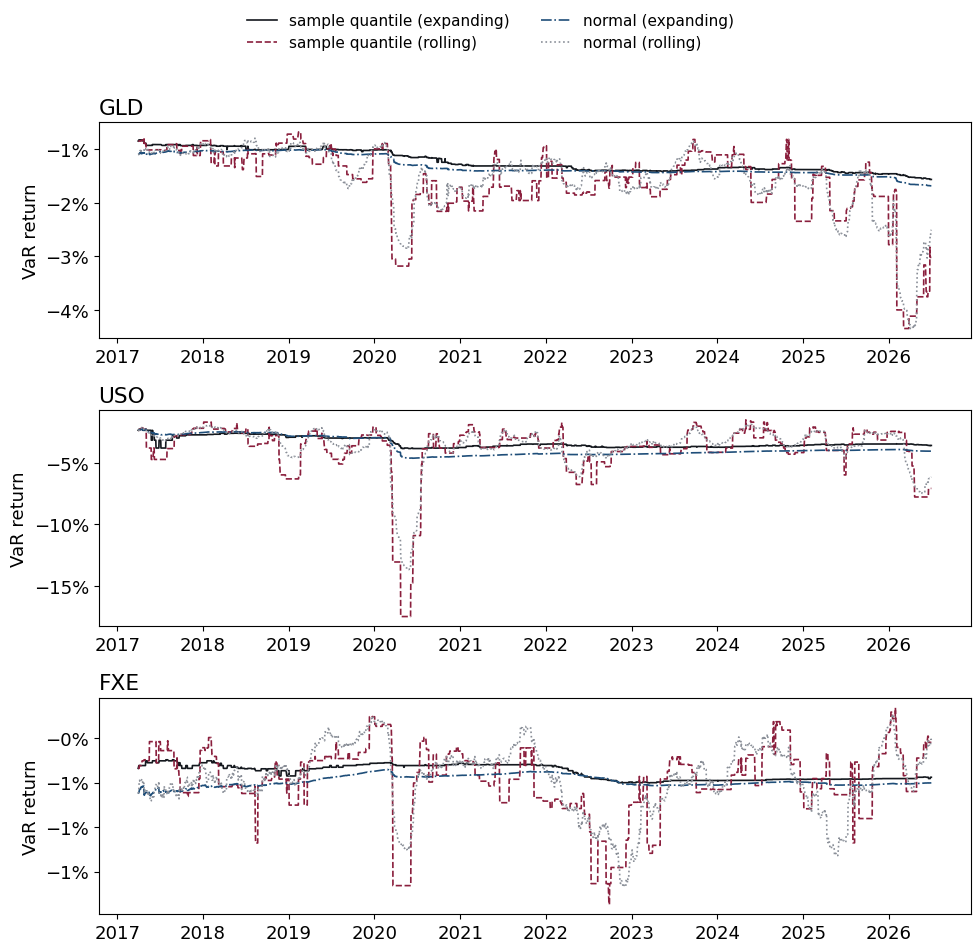
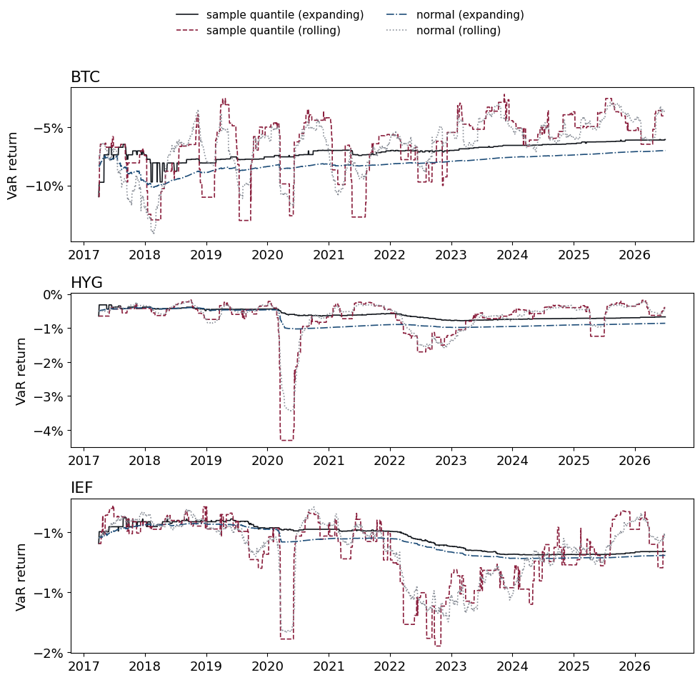
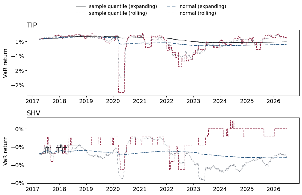
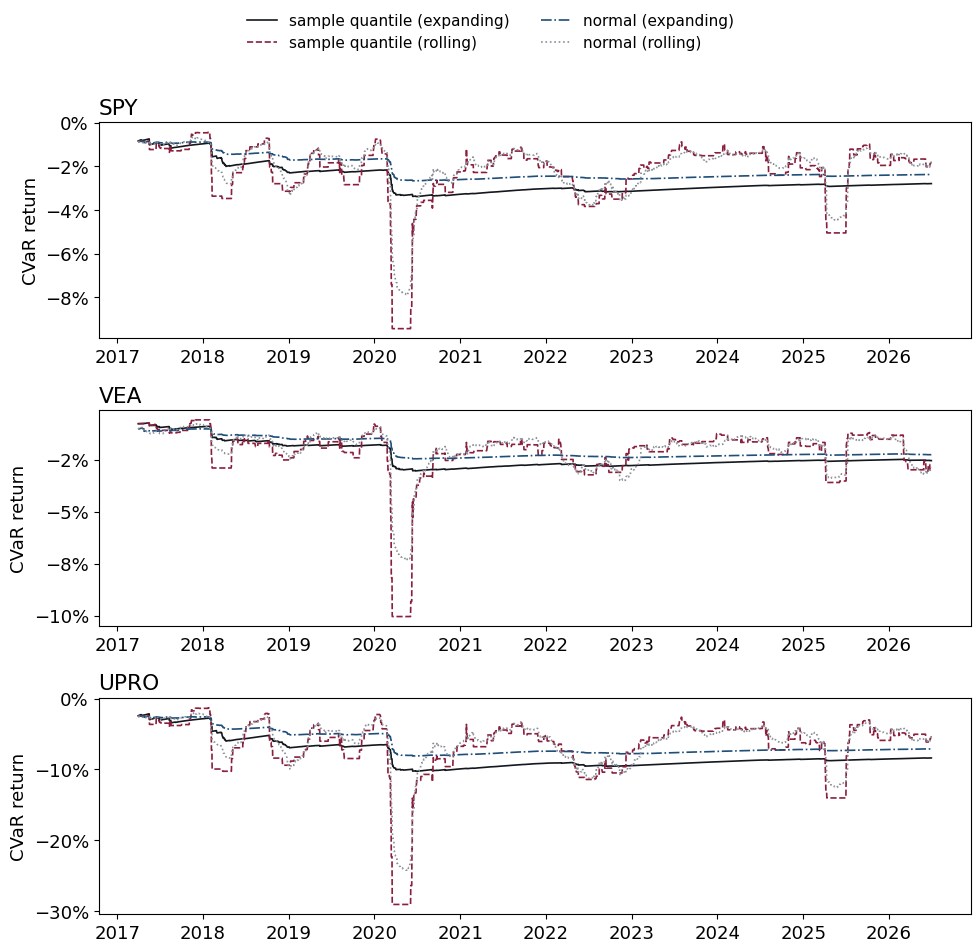
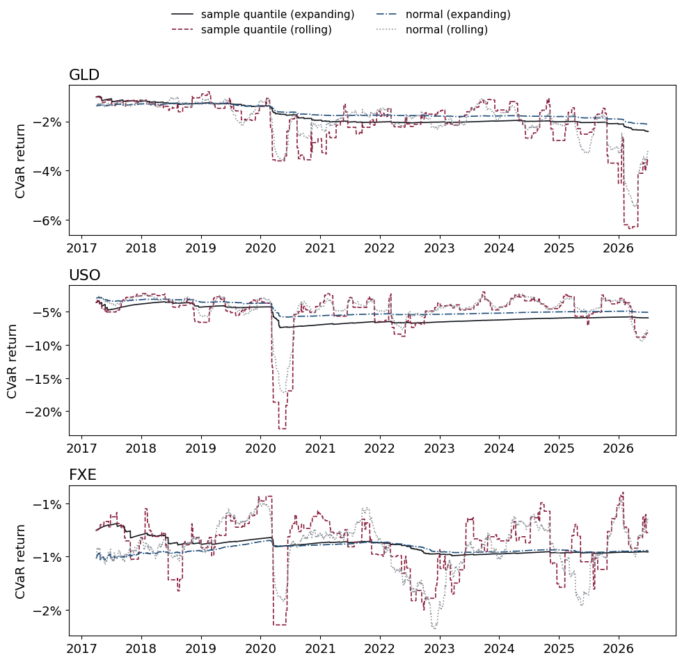
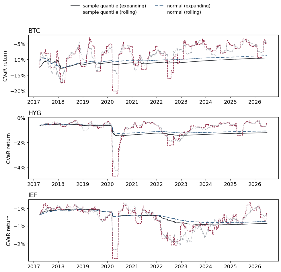
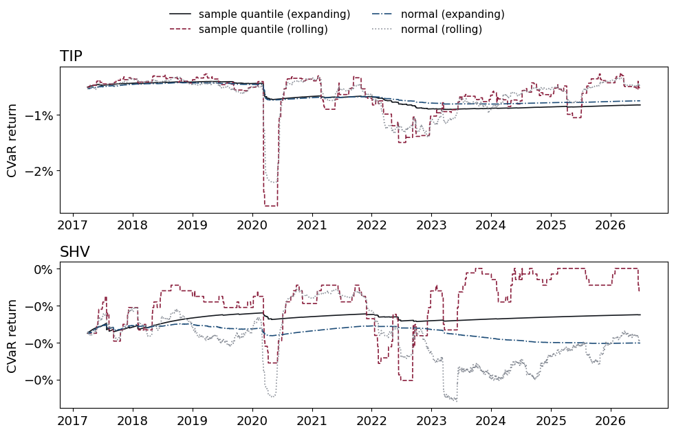
Compare sample-quantile and normal VaR forecasts using expanding and rolling windows. Each forecast uses returns observed before the forecast date.

import pandas as pd
import numpy as np
import matplotlib.pyplot as plt
from matplotlib.ticker import PercentFormatter
from scipy.stats import norm
%matplotlib inline
plt.rcParams['figure.figsize'] = (10, 5)
plt.rcParams['font.size'] = 13
plt.rcParams['legend.fontsize'] = 11

def tail_mean(values, q):
    """Mean of the lowest q probability mass of an empirical distribution."""
    x = np.sort(np.asarray(values, dtype=float))
    mass = q * len(x)
    whole = int(np.floor(mass))
    fraction = mass - whole
    total = x[:whole].sum()
    if fraction > 0:
        total += fraction * x[whole]
    return total / mass

LOADETF = '../data/risk_etf_data.xlsx'
px = pd.read_excel(LOADETF, sheet_name='prices').set_index('Date').dropna()
rets = px.pct_change(fill_method=None).dropna()

FREQ = 252
WINDOW = 60
QUANTILE = .05
mu = 0

Conditional Moments

Conditional VaR uses information available at the forecast date. Under a normal model with zero mean, it depends on the conditional volatility forecast.

The Mean

The normal forecasts below set the conditional mean to zero. The volatility formulas therefore use the second moment, \(\E[r^2]\).

Why might this approximation be useful for daily returns?

With a model for the mean, apply the volatility formulas to the demeaned returns and add the mean forecast when calculating VaR.

Forecast Timing

\(\sigma_t^2\) denotes the variance forecast for day \(t\), using returns through \(t-1\). The formulas below assume a zero conditional mean.

Expanding Window

\[\sigma_t^2=\frac{1}{t-1}\sum_{i=1}^{t-1}r_i^2.\]

Rolling Window

\[\sigma_t^2=\frac{1}{m}\sum_{i=1}^{m}r_{t-i}^2.\]

EWMA

The exponentially weighted moving average (EWMA) gives more weight to recent returns. For \(0<\lambda<1\),

\[\sigma_t^2=\lambda\sigma_{t-1}^2+(1-\lambda)r_{t-1}^2.\]

Starting from \(\sigma_1^2\), the equivalent finite-history expression is

\[\sigma_t^2=\lambda^{t-1}\sigma_1^2+ (1-\lambda)\sum_{i=1}^{t-1}\lambda^{i-1}r_{t-i}^2.\]

The initial variance and return weights sum to one.

GARCH

\[\sigma_t^2=\alpha_0+\gamma_1\sigma_{t-1}^2+\alpha_1r_{t-1}^2.\]

For GARCH(1,1), \(\alpha_0>0\) and \(\alpha_1,\gamma_1\ge0\). The condition \(\alpha_1+\gamma_1<1\) gives a finite unconditional variance. Additional lags give higher-order GARCH models.

Comparing Forecasts

Use daily ETF price returns for four forecasts:

Distribution estimate	Expanding window	Rolling window
Sample quantile	All prior returns	Most recent returns
Normal	Expanding second moment; zero mean	Rolling second moment; zero mean

The setup table specifies the window and initial sample. All methods are evaluated on the same dates. EWMA and GARCH are defined above for comparison; the filtered-historical-simulation page applies GARCH.

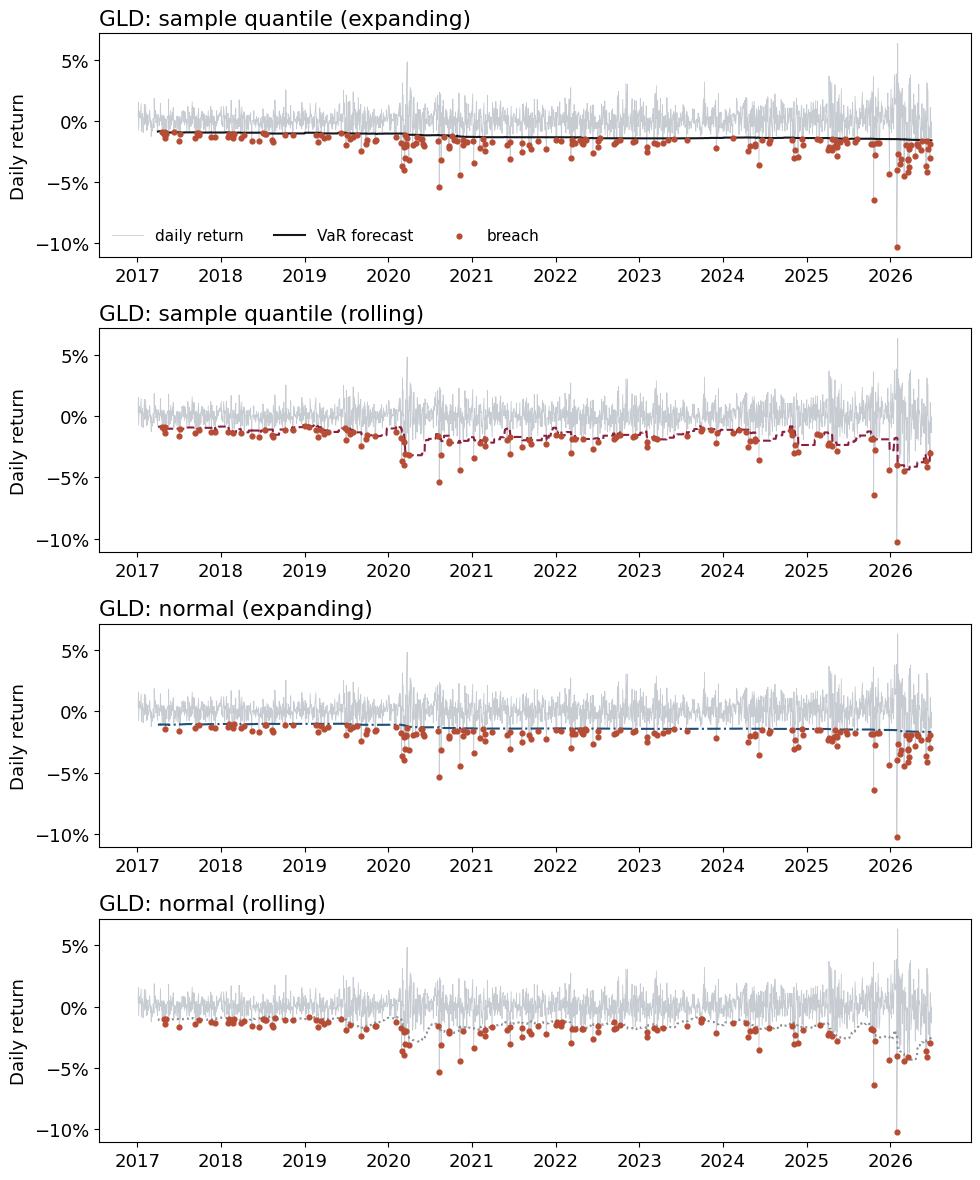
A breach occurs when the realized return falls below the forecast quantile. Compare breach rates with the target and inspect whether breaches cluster.

METHODS = ['sample quantile (expanding)', 'sample quantile (rolling)',
           'normal (expanding)', 'normal (rolling)']
COLORS = ['#14181e', '#8a1f3d', '#1f4e79', '#8a8f98']
STYLES = ['-', '--', '-.', ':']

sigma_expanding = np.sqrt(rets.pow(2).expanding(WINDOW).mean())
sigma_rolling = np.sqrt(rets.pow(2).rolling(WINDOW).mean())
setup = pd.DataFrame({'Rolling window, days': [WINDOW],
                      'Minimum history, days': [WINDOW],
                      'Target breach rate': [QUANTILE]})
display(setup.style.set_table_attributes('class="dataframe"').hide(axis='index').format(
    {'Rolling window, days': '{:,.0f}', 'Minimum history, days': '{:,.0f}',
     'Target breach rate': '{:.0%}'}, na_rep='').set_caption('Forecast setup'))

Forecast setup

Rolling window, days	Minimum history, days	Target breach rate
60	60	5%

sample_quantile = lambda x: np.quantile(x, QUANTILE, method='inverted_cdf')
sample_tail_mean = lambda x: tail_mean(x, QUANTILE)
zscore = norm.ppf(QUANTILE)

# Index each estimate by its target return date.
VaRret = {
    METHODS[0]: rets.expanding(WINDOW).apply(sample_quantile, raw=True).shift(1),
    METHODS[1]: rets.rolling(WINDOW).apply(sample_quantile, raw=True).shift(1),
    METHODS[2]: (mu + zscore*sigma_expanding).shift(1),
    METHODS[3]: (mu + zscore*sigma_rolling).shift(1),
}
CVaRret = {
    METHODS[0]: rets.expanding(WINDOW).apply(sample_tail_mean, raw=True).shift(1),
    METHODS[1]: rets.rolling(WINDOW).apply(sample_tail_mean, raw=True).shift(1),
    METHODS[2]: (mu - norm.pdf(zscore)/QUANTILE*sigma_expanding).shift(1),
    METHODS[3]: (mu - norm.pdf(zscore)/QUANTILE*sigma_rolling).shift(1),
}

# One asset per row keeps the four forecast series readable at book width.
for measure, estimates in [('VaR', VaRret), ('CVaR', CVaRret)]:
    for start in range(0, len(rets.columns), 3):
        tickers = rets.columns[start:start+3]
        fig, axes = plt.subplots(len(tickers), 1, figsize=(10, 3.2*len(tickers)),
                                 squeeze=False)
        for ax, tick in zip(axes[:, 0], tickers):
            for method, color, style in zip(METHODS, COLORS, STYLES):
                ax.plot(rets.index, estimates[method][tick], label=method,
                        color=color, ls=style, lw=1.2)
            ax.set_title(tick, loc='left')
            ax.set_ylabel(f'{measure} return')
            ax.yaxis.set_major_formatter(PercentFormatter(1, decimals=0))
        handles, labels = axes[0, 0].get_legend_handles_labels()
        fig.legend(handles, labels, loc='upper center', ncol=2, frameon=False)
        fig.tight_layout(rect=(0, 0, 1, .92))
        plt.show()

valid = rets.notna()
for method in METHODS:
    valid &= VaRret[method].notna()
hits = {method: (rets < VaRret[method]).astype(float).where(valid) for method in METHODS}
hitratio = pd.DataFrame({method: hits[method].sum()/valid.sum() for method in METHODS})

ax = hitratio.plot.bar(figsize=(10, 5), color=COLORS, rot=0)
ax.axhline(QUANTILE, color='#b64c33', ls='--', lw=1, label='target')
ax.set_title('VaR Breach Rates by Asset', loc='left')
ax.set_ylabel('Breach rate')
ax.yaxis.set_major_formatter(PercentFormatter(1, decimals=0))
ax.legend(loc='upper center', bbox_to_anchor=(.5, 1.28), ncol=2, frameon=False)
plt.show()

display(hitratio.style.set_table_attributes('class="dataframe"').format({m: '{:.1%}' for m in METHODS}, na_rep='').set_caption(
    'Breach rates on common forecast dates; target 5%'))

Breach rates on common forecast dates; target 5%

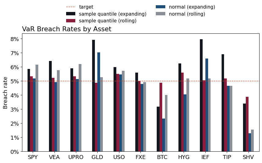
	sample quantile (expanding)	sample quantile (rolling)	normal (expanding)	normal (rolling)
SPY	5.9%	5.3%	5.2%	6.2%
VEA	6.4%	5.2%	4.9%	5.8%
UPRO	5.9%	5.3%	5.1%	6.2%
GLD	7.9%	4.9%	7.0%	5.2%
USO	6.0%	5.5%	5.5%	5.7%
FXE	5.6%	5.0%	4.8%	4.9%
BTC	3.2%	4.9%	2.3%	4.0%
HYG	6.2%	5.6%	4.0%	5.2%
IEF	8.0%	5.0%	6.6%	5.2%
TIP	6.9%	5.2%	4.6%	4.6%
SHV	3.4%	3.9%	1.3%	1.5%

# RMSE is in percentage points; lower values indicate closer average calibration.
calibration = pd.DataFrame({
    'Calibration RMSE, pp': np.sqrt(((hitratio-QUANTILE)**2).mean())*100,
    'Forecast days per asset': int(valid.sum().iloc[0]),
})
calibration.style.set_table_attributes('class="dataframe"').format({'Calibration RMSE, pp': '{:.2f}',
                         'Forecast days per asset': '{:,.0f}'}, na_rep='').set_caption(
    'Root mean squared breach-rate deviation across assets')

Root mean squared breach-rate deviation across assets

	Calibration RMSE, pp	Forecast days per asset
sample quantile (expanding)	1.73	2,324
sample quantile (rolling)	0.45	2,324
normal (expanding)	1.62	2,324
normal (rolling)	1.24	2,324

tick = 'GLD'
fig, axes = plt.subplots(len(METHODS), 1, figsize=(10, 12))
for ax, method, color, style in zip(axes, METHODS, COLORS, STYLES):
    forecast = VaRret[method][tick]
    breached = valid[tick] & (rets[tick] < forecast)
    ax.plot(rets.index, rets[tick], color='#c7ccd2', lw=.6, label='daily return')
    ax.plot(rets.index, forecast, color=color, ls=style, label='VaR forecast')
    ax.scatter(rets.index[breached], rets.loc[breached, tick],
               color='#b64c33', s=12, label='breach', zorder=3)
    ax.set_title(f'{tick}: {method}', loc='left')
    ax.set_ylabel('Daily return')
    ax.yaxis.set_major_formatter(PercentFormatter(1, decimals=0))
axes[0].legend(ncol=3, frameon=False)
fig.tight_layout()
plt.show()

Historical Simulation

Historical simulation uses the empirical distribution of portfolio returns or losses. The sample quantile gives VaR without imposing a normal distribution.

An expanding window uses all available history. A rolling window limits the sample to recent observations. Neither explicitly models volatility dynamics; filtered historical simulation adds that adjustment.

CVaR

Sort \(N\) observations from lowest to highest, \(r_{(1)},\ldots,r_{(N)}\). Let \(k=\lfloor qN\rfloor\) and \(a=qN-k\). The empirical lower-tail mean is

\[r^{\CVaR_{q,1}}=\frac{\sum_{i=1}^k r_{(i)}+a\,r_{(k+1)}}{qN}.\]

Omit the last term when \(a=0\). This averages exactly the worst \(q\) probability mass and handles a sample size for which \(qN\) is not an integer.

Sample Size

The empirical distribution preserves observed skewness and tail outcomes. Its tail estimates depend on the number of observations near the quantile.

How many observations fall in the tail at the chosen probability and window?

Changing Distributions

Longer windows provide more tail observations but may combine different market conditions. Shorter windows use more recent data and give less precise tail estimates.

Resampling individual dates treats historical shocks as exchangeable. Remaining serial dependence or changes in the shock distribution require additional modeling.

Monte Carlo Simulation

1. Draw risk factors from a statistical model.

2. Revalue the portfolio under each draw.

3. Calculate VaR and CVaR from the simulated PnL distribution.

Simulation permits nonlinear valuation and dynamics without requiring a closed-form distribution for portfolio PnL.

Bonds and Options

• Simulate stock prices and other option-pricing inputs, then revalue the options at the shorter remaining maturity.

• Simulate yield-curve changes, then reprice each bond’s cash flows.

Other Distribution Models

• Student’s t. Allows heavier tails than a normal distribution. Forecast performance depends on the fitted parameters and volatility model.

• Extreme value theory. Models tail behavior beyond a chosen threshold.

• Quantile regression. Estimates a conditional quantile directly from predictors.