LFD for Dimension Reduction

With more stocks than weekly observations, the sample covariance matrix is singular. We decompose S&P 500 stock returns using sector ETFs as factors.

The Panel

import pandas as pd
import numpy as np
import matplotlib.pyplot as plt
from matplotlib.ticker import PercentFormatter
from matplotlib.colors import LinearSegmentedColormap
from sklearn.decomposition import PCA
from IPython.display import display
%matplotlib inline
plt.rcParams['figure.figsize'] = (10, 5)
plt.rcParams['font.size'] = 15

FREQ = 52

stocks = pd.read_excel('../data/spx_returns_weekly_legacy_2025.xlsx',
                       sheet_name='s&p500 rets').set_index('date')
sectors = pd.read_excel('../data/sector_etf_data.xlsx',
                        sheet_name='total returns').set_index('date')

# Use the same complete observations and stocks for both factor models.
dates = stocks.index.intersection(sectors.dropna().index)
stocks = stocks.loc[dates].dropna(axis=1)
F = sectors.loc[dates]

panel = pd.Series({
    'Stocks': stocks.shape[1],
    'Sector factors': F.shape[1],
    'Weekly observations': len(dates),
    'First date': dates.min().strftime('%Y-%m-%d'),
    'Last date': dates.max().strftime('%Y-%m-%d'),
}, name='Sample')
panel.to_frame().style.format(na_rep='').set_caption('The estimation panel')

The estimation panel

	Sample
Stocks	442
Sector factors	11
Weekly observations	361
First date	2018-06-29
Last date	2025-05-23

Sector ETF Factors

The sector ETFs provide tradable factor exposures. For stock \(i\), let \(r_{i,t}\) denote its return and \(f_t\) the vector of sector ETF returns:

\[ r_{i,t} = \alpha_i + \beta_i' f_t + \epsilon_{i,t}. \]

The intercept is \(\alpha_i\), the factor loadings are \(\beta_i\), and \(\epsilon_{i,t}\) is the residual. We estimate a separate regression for each stock.

Let \(B\) collect the loading vectors \(\beta_i\) as columns. OLS gives the sample covariance relation

\[ \Sigma_r = B'\Sigma_f B + \Sigma_\epsilon, \]

where \(\Sigma_f\) is the factor covariance matrix and \(\Sigma_\epsilon\) is the residual covariance matrix. Approximating \(\Sigma_\epsilon\) by the diagonal matrix \(D\) of residual variances gives

\[ \Sigma_r \approx B'\Sigma_f B + D. \]

We then estimate factor covariances, stock loadings, and residual variances. The diagonal approximation drops residual covariances. Its adequacy depends on portfolio exposures.

def fit_factors(returns, factors):
    X = np.column_stack([np.ones(len(factors)), factors.values])
    coef = np.linalg.lstsq(X, returns.values, rcond=None)[0]
    residuals = pd.DataFrame(returns.values - X @ coef,
                             index=returns.index, columns=returns.columns)
    r2 = 1 - residuals.var() / returns.var()
    return coef[0], coef[1:], residuals, r2

alpha, B, E, R2 = fit_factors(stocks, F)

# Keep the same exposure-based ordering in every heatmap.
groups = pd.Series(F.columns[np.abs(B).argmax(axis=0)], index=stocks.columns)
ordered = pd.DataFrame({'ETF': groups, 'Stock': stocks.columns}).sort_values(['ETF', 'Stock'])
stock_order = ordered.index
sizes = ordered.groupby('ETF', sort=False).size()
group_ticks = sizes.cumsum().to_numpy() - sizes.to_numpy() / 2 - 0.5


def pairwise(df):
    corr = df.corr().to_numpy()
    return corr[np.triu_indices_from(corr, k=1)]


def mean_abs_corr(df):
    return np.abs(pairwise(df)).mean()


def heatmap(df, title):
    corr = df.loc[:, stock_order].corr().to_numpy()
    corr = np.ma.array(corr, mask=np.eye(len(corr), dtype=bool))
    fig, ax = plt.subplots(figsize=(8.5, 7.5), layout='constrained')
    cmap = LinearSegmentedColormap.from_list(
        'correlation', plt.get_cmap('RdBu_r')(np.linspace(0.45, 1, 256)))
    im = ax.imshow(corr, cmap=cmap, vmin=-0.1, vmax=1,
                   interpolation='nearest', aspect='equal')
    ax.set_xticks(group_ticks, sizes.index, rotation=90)
    ax.set_yticks(group_ticks, sizes.index)
    ax.tick_params(axis='both', labelsize=13)
    ax.set_xlabel('Stocks grouped by ETF loading')
    ax.set_title(title, loc='left')
    fig.colorbar(im, ax=ax, shrink=0.8, label='Correlation',
                 extend='min', ticks=[-0.1, 0, 0.25, 0.5, 0.75, 1],
                 format=PercentFormatter(1, decimals=0))
    plt.show()


def show_fit(r2):
    fig, ax = plt.subplots(layout='constrained')
    ax.hist(r2, bins=np.linspace(0, 1, 41), color='gray', alpha=0.75)
    ax.axvline(r2.median(), color='black', lw=2, label='Median')
    ax.set_xlim(0, 1)
    ax.xaxis.set_major_formatter(PercentFormatter(1))
    ax.set_xlabel('Regression $R^2$')
    ax.set_ylabel('Stocks')
    ax.legend()
    plt.show()
    fit = pd.Series({
        'Mean': r2.mean(),
        'Median': r2.median(),
        f'Minimum ({r2.idxmin()})': r2.min(),
        f'Maximum ({r2.idxmax()})': r2.max(),
    }, name='Explained variance')
    display(fit.to_frame().style.format({'Explained variance': '{:.1%}'}, na_rep='')
            .set_caption('Regression fit across stocks'))


def show_correlations(residuals):
    summary = pd.DataFrame({
        'Mean absolute correlation': [mean_abs_corr(stocks), mean_abs_corr(residuals)]
    }, index=['Returns', 'Residuals'])
    display(summary.style.format({'Mean absolute correlation': '{:.1%}'}, na_rep='')
            .set_caption('Unique stock pairs, excluding the diagonal'))


def show_risk(residuals):
    vol_r = stocks.std() * np.sqrt(FREQ)
    vol_e = residuals.std() * np.sqrt(FREQ)
    lim = [0, 1.04 * vol_r.max()]
    fig, ax = plt.subplots(figsize=(7.5, 6), layout='constrained')
    ax.plot(lim, lim, color='black', lw=1, ls='--', label='No reduction')
    ax.scatter(vol_r, vol_e, s=18, color='gray', alpha=0.6)
    ax.xaxis.set_major_formatter(PercentFormatter(1))
    ax.yaxis.set_major_formatter(PercentFormatter(1))
    ax.set_xlim(lim)
    ax.set_ylim(lim)
    ax.set_xlabel('Annualized return volatility')
    ax.set_ylabel('Annualized residual volatility')
    ax.legend()
    plt.show()
    shape = pd.DataFrame({
        'Returns': [vol_r.mean(), stocks.skew().mean(), stocks.kurtosis().mean()],
        'Residuals': [vol_e.mean(), residuals.skew().mean(), residuals.kurtosis().mean()],
    }, index=['Annualized volatility', 'Skewness', 'Excess kurtosis'])
    display(shape.T.style.format({'Annualized volatility': '{:.1%}', 'Skewness': '{:.2f}',
                                  'Excess kurtosis': '{:.2f}'}, na_rep='')
            .set_caption('Cross-sectional averages'))


def cumulative_variance(df):
    p = PCA(svd_solver='full').fit(df)
    return p.explained_variance_ratio_.cumsum()


raw_pca = PCA(svd_solver='full').fit(stocks)
cv_raw = raw_pca.explained_variance_ratio_.cumsum()


def show_concentration(residuals):
    cv_resid = cumulative_variance(residuals)
    n = min(20, len(cv_raw), len(cv_resid))
    grid = np.arange(1, n + 1)
    fig, ax = plt.subplots(layout='constrained')
    ax.plot(grid, cv_raw[:n], color='black', lw=2, marker='o', ms=4,
            label='Stock returns')
    ax.plot(grid, cv_resid[:n], color='#b64c33', lw=2, ls='--', marker='s', ms=4,
            label='Residuals')
    ax.set_xlim(1, n)
    ax.set_ylim(0, 1)
    ax.set_xticks(grid[::2])
    ax.yaxis.set_major_formatter(PercentFormatter(1))
    ax.set_xlabel('Principal components')
    ax.set_ylabel('Cumulative variance explained')
    ax.legend()
    plt.show()
    cuts = np.array([i for i in (1, 3, 10, 20) if i <= n])
    summary = pd.DataFrame({'Returns': cv_raw[cuts - 1], 'Residuals': cv_resid[cuts - 1]},
                           index=['PC1' if i == 1 else f'First {i}' for i in cuts])
    display(summary.style.format({'Returns': '{:.1%}', 'Residuals': '{:.1%}'}, na_rep='')
            .set_caption('Share of each panel’s total variance'))

Explained Variance

The regression \(R^2\) measures the share of a stock’s return variance explained by the factors.

show_fit(R2)

Regression fit across stocks

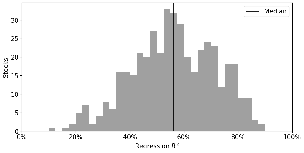
	Explained variance
Mean	56.3%
Median	56.2%
Minimum (ERIE)	12.2%
Maximum (XOM)	89.8%

Pairwise Correlations

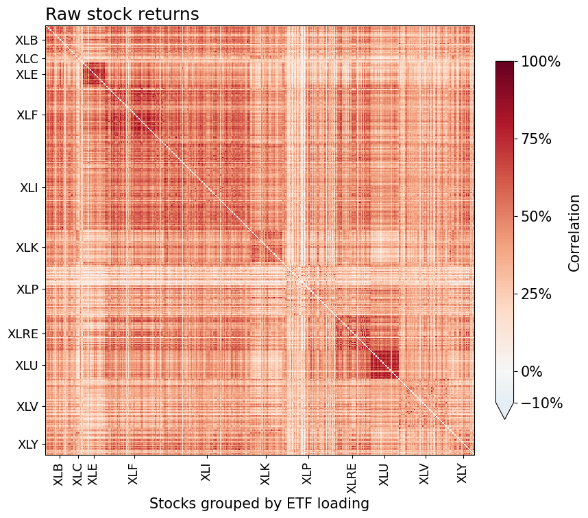
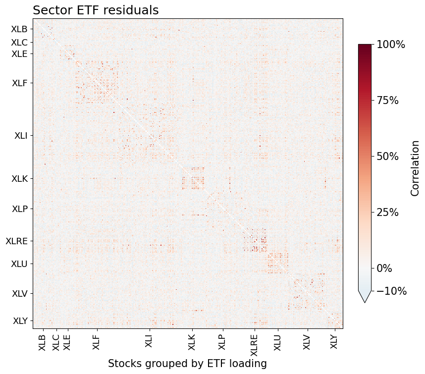
Stocks are grouped by the sector ETF with the largest absolute fitted loading, then alphabetically within each group. All heatmaps use this ordering and the same color scale. The diagonal is omitted.

Values below −10% share the lower-limit color. The correlation quantiles report the full range.

heatmap(stocks, 'Raw stock returns')
heatmap(E, 'Sector ETF residuals')
show_correlations(E)

Unique stock pairs, excluding the diagonal

	Mean absolute correlation
Returns	39.0%
Residuals	6.7%

The mean uses absolute correlations so positive and negative values cannot cancel. A small mean absolute correlation does not establish independence or rule out concentrated residual exposures.

Residual Risk

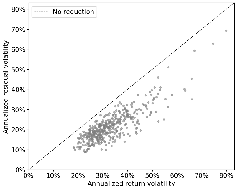
OLS reduces in-sample variance by construction. The comparison measures the remaining variation.

show_risk(E)

Cross-sectional averages

	Annualized volatility	Skewness	Excess kurtosis
Returns	33.1%	0.00	5.46
Residuals	21.6%	0.08	4.37

Substantial excess kurtosis remains after removing sector exposures. Near-zero average skewness can mask skewness in individual stocks.

Variance Concentration

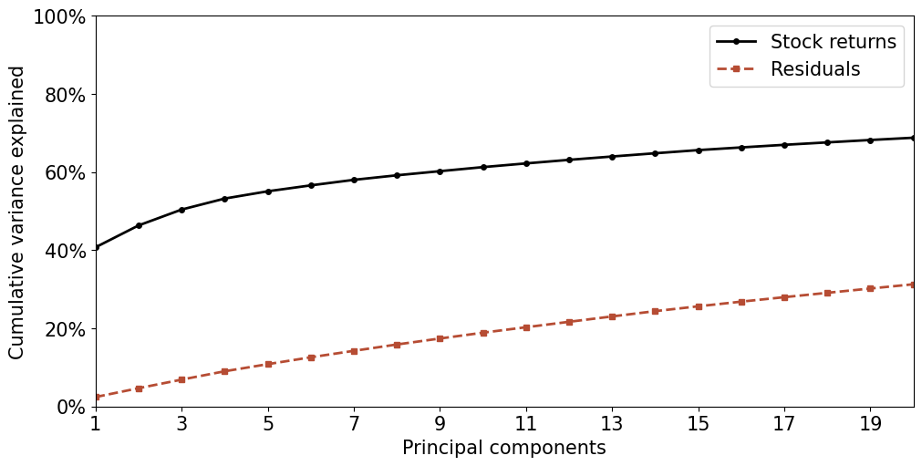
Principal component analysis (PCA) forms uncorrelated linear combinations, ordered by variance. We demean each series without scaling its volatility, so this is PCA of the covariance matrix.

Here, PCA diagnoses the concentration of variance in returns and residuals. The regression factors are still sector ETFs. Each curve divides by the total variance of its own panel.

show_concentration(E)

Share of each panel’s total variance

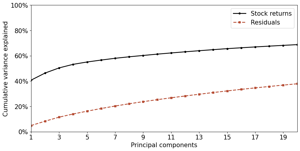
	Returns	Residuals
PC1	40.7%	4.9%
First 3	50.4%	11.5%
First 10	61.3%	25.3%
First 20	68.8%	37.9%

PCA Factors

PCA can also supply the factors. Let \(r_t\) be the vector of stock returns and \(\bar r\) its sample mean. If \(v_j\) is the unit eigenvector associated with the \(j\)th largest eigenvalue of the return covariance matrix, the factor score is

\[ f^{\mathrm{PCA}}_{j,t} = v_j'(r_t - \bar r). \]

We retain the same number of principal components as sector ETFs and use these scores in the same stock regressions and covariance decomposition.

PCA chooses the linear combinations that capture the most total variance in this sample for the given factor count. The factors are estimated from the stocks being explained. We continue to use demeaned returns without volatility scaling.

K = F.shape[1]
F_pca = pd.DataFrame(raw_pca.transform(stocks)[:, :K], index=stocks.index,
                     columns=[f'PC{i}' for i in range(1, K + 1)])
alpha_pca, B_pca, E_pca, R2_pca = fit_factors(stocks, F_pca)

pd.DataFrame({'Factors': [F.shape[1], F_pca.shape[1]]},
             index=['Sector ETFs', 'PCA']).style.format(
    {'Factors': '{:.0f}'}, na_rep=''
).set_caption('Factor counts')

Factor counts

	Factors
Sector ETFs	11
PCA	11

Explained Variance

Apply the same regression fit measures to the PCA factors.

show_fit(R2_pca)

Regression fit across stocks

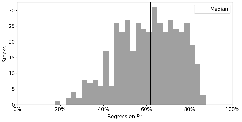
	Explained variance
Mean	60.5%
Median	61.8%
Minimum (ERIE)	18.2%
Maximum (PRU)	87.2%

Pairwise Correlations

Stock residual correlations after removing PCA factors. Ordering and color scale match the earlier heatmaps.

heatmap(E_pca, 'PCA residuals')
show_correlations(E_pca)

Unique stock pairs, excluding the diagonal

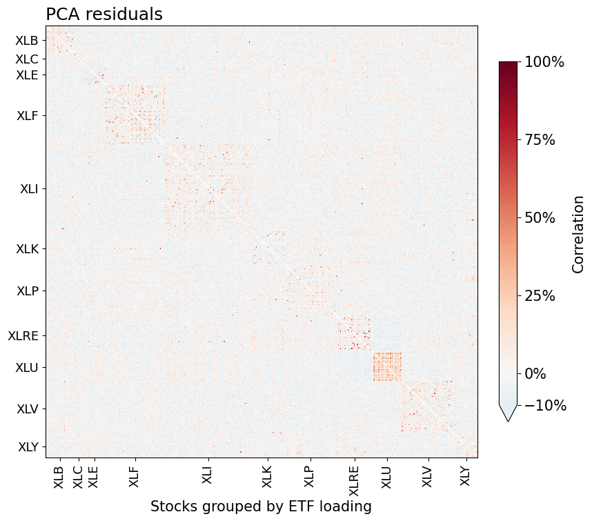
	Mean absolute correlation
Returns	39.0%
Residuals	5.8%

Uncorrelated PCA factors do not imply uncorrelated stock residuals.

Residual Risk

show_risk(E_pca)

Cross-sectional averages

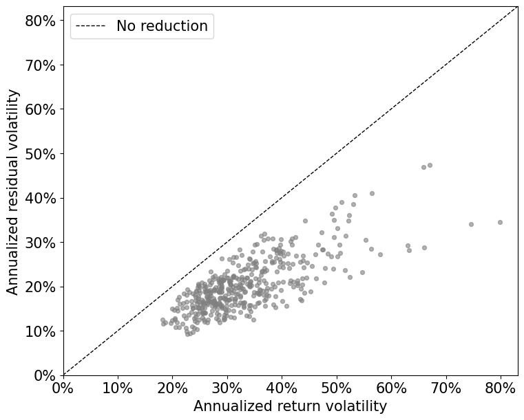
	Annualized volatility	Skewness	Excess kurtosis
Returns	33.1%	0.00	5.46
Residuals	20.2%	0.02	4.17

Variance Concentration

Fit PCA to the remaining residuals to measure how concentrated their variance is. Each curve again uses its own panel’s total variance as the denominator.

show_concentration(E_pca)

Share of each panel’s total variance

	Returns	Residuals
PC1	40.7%	2.4%
First 3	50.4%	6.9%
First 10	61.3%	18.9%
First 20	68.8%	31.3%

Factor Comparison

Mean stock \(R^2\) weights stocks equally. The share of total variance explained weights them by their return variance, which is the criterion PCA maximizes.

The correlation column compares raw returns with residuals from each factor model.

comparison = pd.DataFrame({
    'Raw returns': [np.nan, np.nan, mean_abs_corr(stocks)],
    'Sector ETFs': [R2.mean(), 1 - E.var().sum() / stocks.var().sum(), mean_abs_corr(E)],
    'PCA': [R2_pca.mean(), 1 - E_pca.var().sum() / stocks.var().sum(), mean_abs_corr(E_pca)],
}, index=['Mean stock R²', 'Total variance explained', 'Mean absolute correlation'])
comparison.T.style.format({'Mean stock R²': '{:.1%}', 'Total variance explained': '{:.1%}',
                           'Mean absolute correlation': '{:.1%}'}, na_rep='')\
    .set_caption('In-sample factor comparison')

In-sample factor comparison

	Mean stock R²	Total variance explained	Mean absolute correlation
Raw returns			39.0%
Sector ETFs	56.3%	55.5%	6.7%
PCA	60.5%	62.2%	5.8%

Pairwise Correlation Range

Signed correlations across unique stock pairs, excluding the diagonal. The quantiles use the full correlations, including values below the heatmap scale.

quantiles = pd.DataFrame({
    'Raw returns': np.quantile(pairwise(stocks), [0, 0.25, 0.5, 0.75, 1]),
    'Sector residuals': np.quantile(pairwise(E), [0, 0.25, 0.5, 0.75, 1]),
    'PCA residuals': np.quantile(pairwise(E_pca), [0, 0.25, 0.5, 0.75, 1]),
}, index=['0% (minimum)', '25%', '50% (median)', '75%', '100% (maximum)'])
quantiles.index.name = 'Percentile'
quantiles.style.format({
    'Raw returns': '{:.1%}', 'Sector residuals': '{:.1%}', 'PCA residuals': '{:.1%}'
}, na_rep='').set_caption('Signed pairwise correlation quantiles')

Signed pairwise correlation quantiles

	Raw returns	Sector residuals	PCA residuals
Percentile
0% (minimum)	-12.1%	-45.2%	-38.3%
25%	29.0%	-4.5%	-5.0%
50% (median)	39.2%	0.8%	-0.4%
75%	49.0%	6.3%	4.3%
100% (maximum)	94.6%	86.0%	83.6%

Notes

• Sample. Requiring observations for all sector ETFs limits the sample to the history available for XLC. Only stocks with complete returns over this window are retained.

• Estimation. Both models use the full sample. The calculations treat fitted loadings as fixed and omit estimation uncertainty. PCA’s in-sample variance advantage does not establish better out-of-sample covariance forecasts.

• Volatility modeling. VaR by Filtered Historical Simulation fits GARCH models to the sector factors and resamples factor shocks and stock residuals jointly by date. It leaves residuals unscaled by a volatility model. Low cross-sectional correlation does not establish constant residual volatility. That notebook uses daily data and re-estimates its own loadings.