


Solution - Statistics of the DFA Factors#
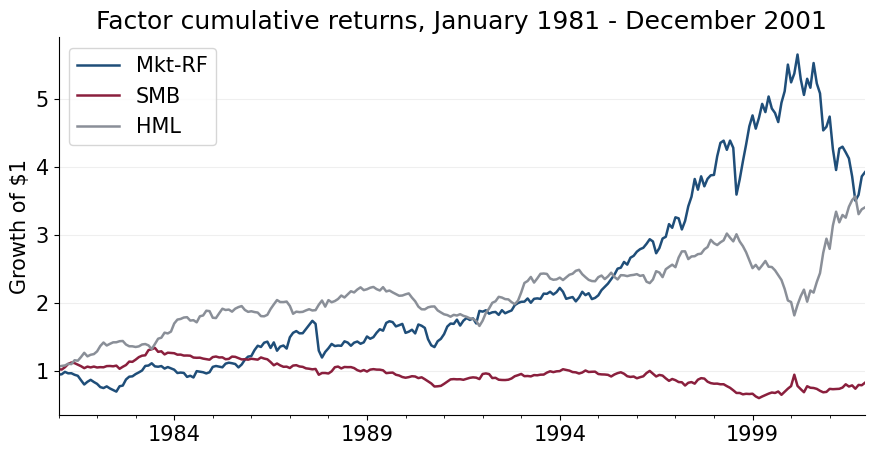
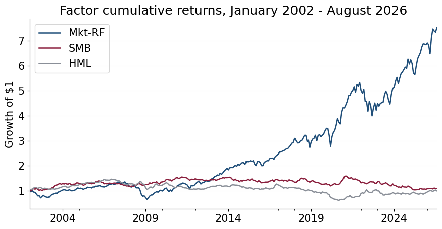
Monthly data through August 2026. Means, volatilities, Sharpe ratios, alphas, Treynor ratios, and information ratios are annualized. VaR is the monthly fifth percentile.
2. Factor statistics#
| Mean | Volatility | Sharpe | Minimum | Maximum | VaR (5%) | |
|---|---|---|---|---|---|---|
| Mkt-RF | 8.10% | 20.50% | 0.39 | -28.74% | 38.81% | -8.41% |
| SMB | 3.39% | 11.43% | 0.30 | -9.89% | 35.96% | -4.19% |
| HML | 5.02% | 13.43% | 0.37 | -13.19% | 35.52% | -4.44% |
| Mean | Volatility | Sharpe | Minimum | Maximum | VaR (5%) | |
|---|---|---|---|---|---|---|
| Mkt-RF | 7.78% | 15.72% | 0.50 | -23.19% | 12.45% | -6.41% |
| SMB | -0.20% | 11.73% | -0.02 | -17.39% | 21.34% | -4.58% |
| HML | 6.44% | 10.98% | 0.59 | -9.73% | 12.25% | -4.17% |
| Mean | Volatility | Sharpe | Minimum | Maximum | VaR (5%) | |
|---|---|---|---|---|---|---|
| Mkt-RF | 9.38% | 15.25% | 0.62 | -17.20% | 13.60% | -7.67% |
| SMB | 0.75% | 8.72% | 0.09 | -5.93% | 7.14% | -3.88% |
| HML | 0.55% | 10.62% | 0.05 | -13.83% | 12.86% | -4.14% |
| Mkt-RF | SMB | HML | |
|---|---|---|---|
| Mkt-RF | 1.00 | 0.37 | 0.44 |
| SMB | 0.37 | 1.00 | 0.31 |
| HML | 0.44 | 0.31 | 1.00 |
| Mkt-RF | SMB | HML | |
|---|---|---|---|
| Mkt-RF | 1.00 | 0.16 | -0.53 |
| SMB | 0.16 | 1.00 | -0.44 |
| HML | -0.53 | -0.44 | 1.00 |
| Mkt-RF | SMB | HML | |
|---|---|---|---|
| Mkt-RF | 1.00 | 0.30 | 0.09 |
| SMB | 0.30 | 1.00 | 0.12 |
| HML | 0.09 | 0.12 | 1.00 |
3. CAPM#
The 25 portfolios use January 1981 through August 2026. Portfolio returns are converted to excess returns before every regression.
| Mean | Volatility | Sharpe | Minimum | Maximum | VaR (5%) | |
|---|---|---|---|---|---|---|
| SMALL LoBM | 1.63% | 27.11% | 0.06 | -34.77% | 35.96% | -12.26% |
| ME1 BM2 | 9.28% | 23.43% | 0.40 | -31.28% | 43.36% | -9.57% |
| ME1 BM3 | 9.62% | 20.03% | 0.48 | -29.19% | 19.90% | -8.44% |
| ME1 BM4 | 11.68% | 19.26% | 0.61 | -28.96% | 25.63% | -7.72% |
| SMALL HiBM | 13.05% | 20.67% | 0.63 | -29.08% | 41.21% | -8.72% |
| ME2 BM1 | 6.61% | 24.37% | 0.27 | -33.08% | 30.24% | -10.25% |
| ME2 BM2 | 10.51% | 20.49% | 0.51 | -32.54% | 19.10% | -8.35% |
| ME2 BM3 | 11.10% | 18.64% | 0.60 | -29.26% | 18.32% | -7.90% |
| ME2 BM4 | 10.97% | 18.10% | 0.61 | -25.26% | 18.69% | -7.50% |
| ME2 BM5 | 11.61% | 21.24% | 0.55 | -32.09% | 25.96% | -9.24% |
| ME3 BM1 | 7.53% | 22.33% | 0.34 | -30.30% | 22.17% | -9.83% |
| ME3 BM2 | 10.67% | 18.65% | 0.57 | -29.08% | 18.67% | -7.82% |
| ME3 BM3 | 9.12% | 17.20% | 0.53 | -25.51% | 16.63% | -7.34% |
| ME3 BM4 | 10.71% | 17.91% | 0.60 | -26.65% | 16.66% | -7.15% |
| ME3 BM5 | 12.53% | 20.13% | 0.62 | -31.39% | 22.91% | -8.37% |
| ME4 BM1 | 9.10% | 19.96% | 0.46 | -26.15% | 25.38% | -8.27% |
| ME4 BM2 | 9.50% | 17.52% | 0.54 | -29.29% | 15.54% | -7.23% |
| ME4 BM3 | 9.71% | 17.34% | 0.56 | -25.14% | 16.81% | -7.54% |
| ME4 BM4 | 10.66% | 17.36% | 0.61 | -32.20% | 16.27% | -6.86% |
| ME4 BM5 | 10.80% | 19.71% | 0.55 | -32.64% | 20.37% | -8.36% |
| BIG LoBM | 9.52% | 16.34% | 0.58 | -22.25% | 14.90% | -7.55% |
| ME5 BM2 | 8.89% | 15.37% | 0.58 | -23.05% | 16.07% | -6.36% |
| ME5 BM3 | 8.60% | 15.25% | 0.56 | -22.63% | 14.25% | -7.10% |
| ME5 BM4 | 7.29% | 16.88% | 0.43 | -27.59% | 16.36% | -7.28% |
| BIG HiBM | 11.77% | 20.86% | 0.56 | -28.58% | 31.37% | -8.85% |
| Beta | Alpha | R-squared | Treynor ratio | Information ratio | |
|---|---|---|---|---|---|
| SMALL LoBM | 1.36 | -10.17% | 0.60 | 1.19% | -0.60 |
| ME1 BM2 | 1.16 | -0.75% | 0.59 | 8.00% | -0.05 |
| ME1 BM3 | 1.05 | 0.56% | 0.65 | 9.18% | 0.05 |
| ME1 BM4 | 0.97 | 3.32% | 0.60 | 12.07% | 0.27 |
| SMALL HiBM | 0.99 | 4.50% | 0.55 | 13.21% | 0.32 |
| ME2 BM1 | 1.33 | -4.92% | 0.72 | 4.96% | -0.38 |
| ME2 BM2 | 1.14 | 0.69% | 0.73 | 9.26% | 0.07 |
| ME2 BM3 | 1.04 | 2.13% | 0.74 | 10.71% | 0.22 |
| ME2 BM4 | 0.97 | 2.60% | 0.68 | 11.34% | 0.26 |
| ME2 BM5 | 1.10 | 2.08% | 0.64 | 10.54% | 0.16 |
| ME3 BM1 | 1.27 | -3.44% | 0.77 | 5.94% | -0.32 |
| ME3 BM2 | 1.08 | 1.30% | 0.81 | 9.85% | 0.16 |
| ME3 BM3 | 0.98 | 0.61% | 0.78 | 9.27% | 0.08 |
| ME3 BM4 | 0.99 | 2.18% | 0.72 | 10.86% | 0.23 |
| ME3 BM5 | 1.05 | 3.47% | 0.65 | 11.96% | 0.29 |
| ME4 BM1 | 1.18 | -1.06% | 0.83 | 7.74% | -0.13 |
| ME4 BM2 | 1.05 | 0.39% | 0.86 | 9.02% | 0.06 |
| ME4 BM3 | 1.00 | 1.04% | 0.80 | 9.68% | 0.13 |
| ME4 BM4 | 0.97 | 2.25% | 0.75 | 10.96% | 0.26 |
| ME4 BM5 | 1.03 | 1.87% | 0.66 | 10.46% | 0.16 |
| BIG LoBM | 1.00 | 0.88% | 0.89 | 9.52% | 0.16 |
| ME5 BM2 | 0.92 | 0.92% | 0.86 | 9.64% | 0.16 |
| ME5 BM3 | 0.87 | 1.07% | 0.78 | 9.87% | 0.15 |
| ME5 BM4 | 0.90 | -0.46% | 0.67 | 8.13% | -0.05 |
| BIG HiBM | 1.05 | 2.73% | 0.60 | 11.26% | 0.21 |
CAPM mean absolute annualized alpha: 2.22%
3. Cross-sectional Estimation#
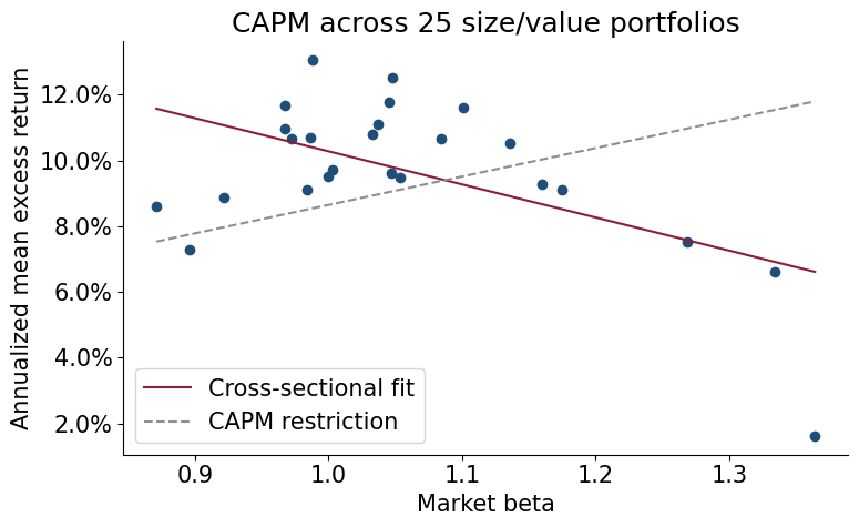
Compare \(\bar{r}^{i} = \eta + \beta^{i}\lambda + \upsilon^{i}\) with \(\eta=0\). The restriction applies to the cross-sectional intercept. Each time-series regression still estimates its own alpha.
Centered \(R^2\) uses \(\sum_i(\bar{r}^{i}-\bar{r})^2\) as its denominator; uncentered \(R^2\) uses \(\sum_i(\bar{r}^{i})^2\). Compare the same definition across columns. statsmodels reports uncentered \(R^2\) by default when the intercept is omitted.
| With intercept | Zero intercept | |
|---|---|---|
| Intercept | 20.34% | 0.00% |
| Market premium | -10.06% | 8.92% |
| Mean market excess return | 8.65% | 8.65% |
| Pricing MAE | 1.41% | 2.09% |
| With intercept | Zero intercept | |
|---|---|---|
| R-squared (centered) | 0.30 | -0.77 |
| R-squared (uncentered) | 0.96 | 0.91 |
5. Joint Test of Alphas#
| Statistic | Degrees of freedom | p-value | |
|---|---|---|---|
| CAPM joint alpha test | 131.76 | 25 | 1.78e-16 |
The joint test uses the residual covariance across all portfolios. Separate t-tests do not account for this covariance or control the overall rejection rate.
Reading the Size of H#
The original investment opportunity is the market, with an annualized Sharpe ratio of 0.56. The expanded investment universe includes the market and all 25 size/value portfolios. Its Sharpe ratio is the maximum obtainable by optimizing their weights.
Our actual CAPM statistic is \(H=131.76\), using \(T=548\) monthly observations.
Quick Approximation#
Convert \(H\) into the annualized information ratio of the optimized market-hedged component:
This drops the small monthly factor-Sharpe correction. Including it raises 1.70 to 1.72. The shortcut is accurate when the factors’ monthly squared Sharpe is small relative to one.
Full Calculation#
Monthly baseline. Convert the market’s squared Sharpe ratio to monthly units:
Squared Sharpe gain. Rearrange the test statistic:
Expanded Sharpe. Annualize the gain, add it to the market’s squared Sharpe ratio, and take the square root:
The optimized combination of market-hedged portfolios has an annualized information ratio of \(\sqrt{12(0.2467)}=1.72\). Its returns are uncorrelated with the market in this regression sample. Combining it optimally with the market gives Sharpe \(\sqrt{0.56^2+1.72^2}=1.81\).
These are in-sample, unconstrained portfolios with shorting and risk-free borrowing or lending allowed. Calculations use monthly covariance matrices with divisor \(T\); displayed inputs are rounded.
4. Beyond CAPM#
| Time-series MAE | Cross-sectional MAE | R-squared | Intercept | |
|---|---|---|---|---|
| Model | ||||
| CAPM | 2.22% | 1.41% | 0.30 | 20.34% |
| Tangency | 0.00% | 0.00% | 1.00 | 0.00% |
| Fama-French 3-factor | 1.38% | 1.15% | 0.48 | 16.75% |
| Tangency | Alpha | |
|---|---|---|
| SMALL LoBM | 0.05 | 0.00% |
| ME1 BM2 | 0.26 | 0.00% |
| ME1 BM3 | 0.27 | 0.00% |
| ME1 BM4 | 0.32 | 0.00% |
| SMALL HiBM | 0.36 | 0.00% |
| ME2 BM1 | 0.18 | 0.00% |
| ME2 BM2 | 0.29 | 0.00% |
| ME2 BM3 | 0.31 | 0.00% |
| ME2 BM4 | 0.30 | 0.00% |
| ME2 BM5 | 0.32 | 0.00% |
| ME3 BM1 | 0.21 | -0.00% |
| ME3 BM2 | 0.30 | 0.00% |
| ME3 BM3 | 0.25 | 0.00% |
| ME3 BM4 | 0.30 | 0.00% |
| ME3 BM5 | 0.35 | 0.00% |
| ME4 BM1 | 0.25 | 0.00% |
| ME4 BM2 | 0.26 | 0.00% |
| ME4 BM3 | 0.27 | 0.00% |
| ME4 BM4 | 0.30 | 0.00% |
| ME4 BM5 | 0.30 | 0.00% |
| BIG LoBM | 0.26 | 0.00% |
| ME5 BM2 | 0.25 | 0.00% |
| ME5 BM3 | 0.24 | 0.00% |
| ME5 BM4 | 0.20 | 0.00% |
| BIG HiBM | 0.33 | 0.00% |
| With intercept | Zero intercept | |
|---|---|---|
| Intercept | 0.00% | 0.00% |
| Tangency premium | 36.10% | 36.10% |
| Pricing MAE | 0.00% | 0.00% |
| With intercept | Zero intercept | |
|---|---|---|
| R-squared (centered) | 1.00 | 1.00 |
| R-squared (uncentered) | 1.00 | 1.00 |
| Mkt-RF | SMB | HML | Alpha | |
|---|---|---|---|---|
| SMALL LoBM | 1.12 | 1.37 | -0.26 | -7.69% |
| ME1 BM2 | 0.96 | 1.33 | -0.01 | 0.57% |
| ME1 BM3 | 0.93 | 1.06 | 0.28 | 0.33% |
| ME1 BM4 | 0.88 | 1.07 | 0.48 | 2.18% |
| SMALL HiBM | 0.93 | 1.06 | 0.69 | 2.41% |
| ME2 BM1 | 1.13 | 1.05 | -0.31 | -2.49% |
| ME2 BM2 | 1.01 | 0.93 | 0.12 | 1.06% |
| ME2 BM3 | 0.99 | 0.73 | 0.39 | 1.06% |
| ME2 BM4 | 0.94 | 0.77 | 0.59 | 0.69% |
| ME2 BM5 | 1.08 | 0.93 | 0.83 | -0.77% |
| ME3 BM1 | 1.10 | 0.77 | -0.35 | -1.12% |
| ME3 BM2 | 1.02 | 0.59 | 0.17 | 1.11% |
| ME3 BM3 | 0.98 | 0.43 | 0.42 | -0.90% |
| ME3 BM4 | 1.01 | 0.46 | 0.64 | -0.28% |
| ME3 BM5 | 1.09 | 0.54 | 0.87 | 0.05% |
| ME4 BM1 | 1.06 | 0.46 | -0.34 | 0.90% |
| ME4 BM2 | 1.05 | 0.23 | 0.21 | -0.32% |
| ME4 BM3 | 1.04 | 0.17 | 0.44 | -0.77% |
| ME4 BM4 | 1.02 | 0.23 | 0.56 | -0.07% |
| ME4 BM5 | 1.12 | 0.26 | 0.86 | -1.74% |
| BIG LoBM | 0.99 | -0.25 | -0.34 | 2.19% |
| ME5 BM2 | 0.96 | -0.20 | 0.09 | 0.33% |
| ME5 BM3 | 0.95 | -0.19 | 0.33 | -0.61% |
| ME5 BM4 | 1.02 | -0.19 | 0.69 | -3.76% |
| BIG HiBM | 1.19 | -0.14 | 0.83 | -1.16% |
| With intercept | Zero intercept | |
|---|---|---|
| Intercept | 16.75% | 0.00% |
| Market premium | -7.91% | 8.00% |
| Size premium | -0.13% | 0.35% |
| Value premium | 3.53% | 3.93% |
| Pricing MAE | 1.15% | 1.41% |
| With intercept | Zero intercept | |
|---|---|---|
| R-squared (centered) | 0.48 | 0.20 |
| R-squared (uncentered) | 0.97 | 0.96 |
The in-sample tangency portfolio has zero pricing errors by construction; that result does not establish out-of-sample performance.
Joint Test of FF3 Alphas#
Test whether all 25 time-series alphas are zero under each model. For FF3, use the mean vector and covariance matrix of all three factors:
Use monthly inputs and covariance matrices with divisor \(T\), matching Problem 3.5. Under the same classical assumptions, the chi-squared reference is asymptotic.
| Statistic | Degrees of freedom | p-value | Mean absolute alpha | |
|---|---|---|---|---|
| CAPM | 131.76 | 25 | 1.78e-16 | 2.22% |
| FF3 | 124.95 | 25 | 2.94e-15 | 1.38% |
FF3 reduces average pricing errors, but both models strongly reject joint zero alphas. The joint test weights alphas by their residual covariance, so smaller average alphas need not produce a proportionately smaller test statistic.
Mean-Variance Comparison#
For FF3, the original investment universe contains Mkt-RF, SMB, and HML. Their best combination has annualized Sharpe 0.71. The expanded universe adds the 25 test portfolios, raising the attainable Sharpe to 1.83.
For \(T\) monthly observations, the annualized information ratio implied by each actual test statistic is
The expanded squared Sharpe is the factor-only squared Sharpe plus this quantity. Sharpe-ratio identity, equation (2).
| Actual H | Factor-only Sharpe | Max information ratio | Expanded Sharpe | |
|---|---|---|---|---|
| Model | ||||
| CAPM | 131.76 | 0.56 | 1.72 | 1.81 |
| FF3 | 124.95 | 0.71 | 1.69 | 1.83 |