VaR: Dynamics and Simulation

This is the companion to Value at Risk (VaR), which defines VaR, CVaR, and coherence.

Here we make VaR operational:

• Conditional moments - model the time-varying volatility that VaR depends on.

• Evaluating VaR - backtest the methods against realized hits.

• Simulation - historical and Monte Carlo approaches, including bonds and options.

import pandas as pd
import numpy as np
import datetime
import warnings

import matplotlib.pyplot as plt
%matplotlib inline
plt.rcParams['figure.figsize'] = (12,6)
plt.rcParams['font.size'] = 15
plt.rcParams['legend.fontsize'] = 13

from matplotlib.ticker import (MultipleLocator,
                               FormatStrFormatter,
                               AutoMinorLocator)

import sys
sys.path.insert(0,'../cmds')
from portfolio import *
from risk import *

LOADETF = '../data/risk_etf_data.xlsx'
px = pd.read_excel(LOADETF,sheet_name='prices').set_index('Date').dropna()

rets = px.pct_change().dropna()

FREQ = 252
WINDOW = 60

QUANTILE = .05
mu = 0

Conditional Moments

Whether using a normal model or something else, we want to allow \(\VaR\) to be dynamic across time. That is, we want the conditional \(\VaR\), utilizing info up to time \(t\).

For normal \(\VaR\) this means having a dynamic model of the volatility.

As mentioned earlier, we typically want conditional versions of any of our risk statistics, so we have broader reasons to want conditional volatility rather than unconditional volatility.

The mean

It will be typical to ignore the mean in the following calculations.

Thus, the formulas calculate the second moment rather than the centered second moment.

Why do you think this convention is often used?

Model for the mean

And note, there is nothing wrong with including the estimated mean in the formulas below (and adjusting the degrees of freedom.)

If using a model for the mean, consider \(r\) in the formulas below as the residual after demeaning.

Notation for the volatility estimates

Below, we use the notation that \(\sigma_t^2\) is estimated using data through \(t-1\) as an estimate of what variance will be the next period (\(t\)).

Expanding

\[\sigma^2_t = \frac{1}{t-1}\sum_{i=1}^{t-1}r^2_i\]

Rolling

\[\sigma^2_t = \frac{1}{m}\sum_{i=1}^mr^2_{t-i}\]

EWMA

The exponential weighted moving average (EWMA) puts more weight on more recent data by setting a geometric decay parameter, \(\lambda\in [0, 1]\). (Typically \(\lambda\) will be in \((.9,1)\).

\[\sigma^2_t = \sum_{i=1}^{\Nt-1} \lambda^{(i-1)} r^2_{t-i}\]

GARCH

\[\sigma^2_t = \alpha_0 + \gamma_1\sigma^2_{t-1} + \alpha_1 r^2_{t-1}\]

GARCH looks a lot like EWMA, but note that

• the parameters do not need to sum to 1

• it could be expanded to take lags of \(r\) or \(\sigma\), which would be a GARCH(2,1), GARCH(1,2), etc.

Evaluating VaR

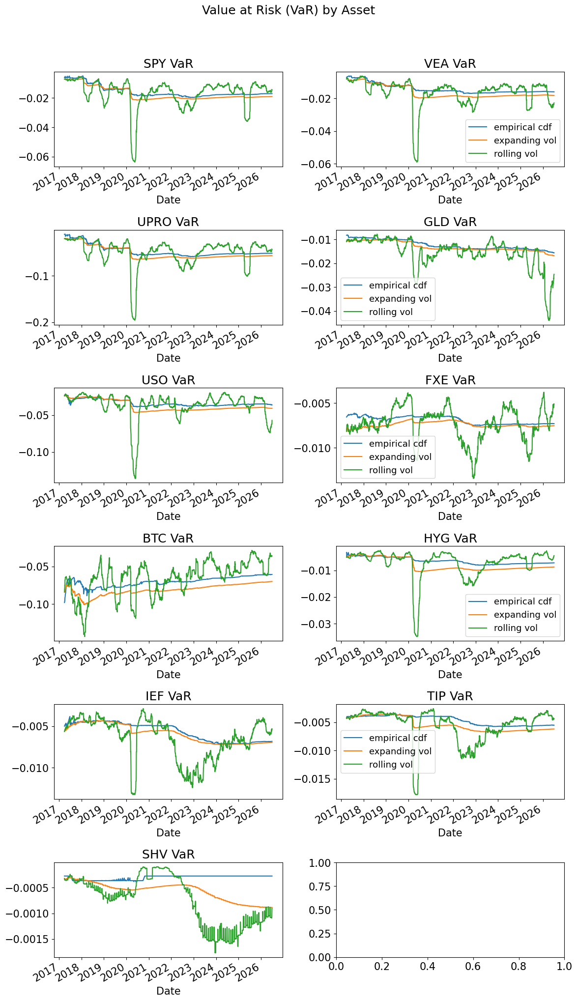
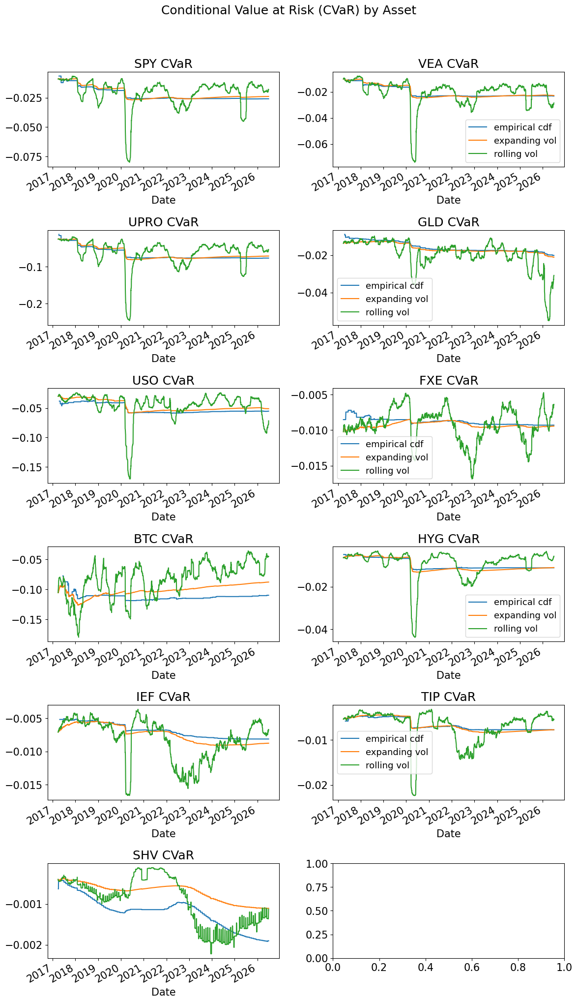
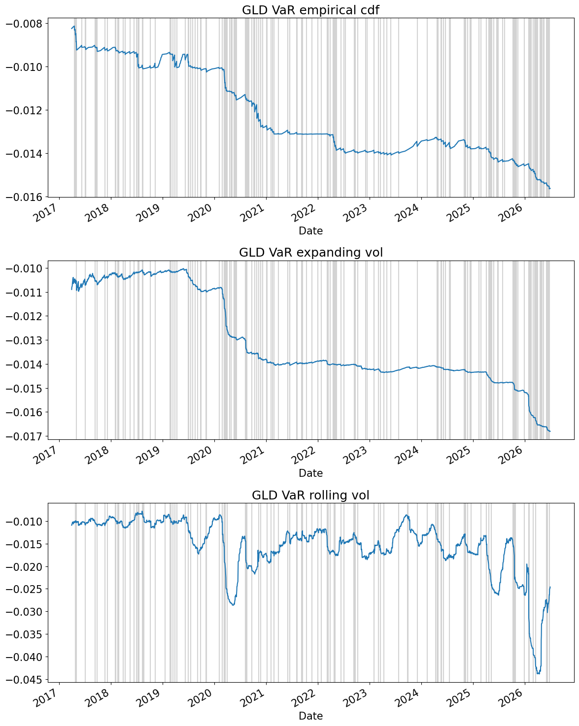
The Hit Test is a common way of backtesting a VaR methodology.

• It checks historically what the daily VaR would have been, given the information known at that time. It compares this to the actual performance for the day.

• If the VaR is working well, then the day-t loss should only exceed the day-\(t\) \(\pnl^{\VaR_{\quant,1}}\) with a probability of \(\quant.\)

• But what if future market environment is very different than past environment with which fit test was run? Many VaR models looked okay before the 2007-2008 crisis hit!

METHODS = ['empirical cdf','expanding vol','rolling vol']

sigma_expanding = rets.expanding(WINDOW).std()
sigma_rolling = rets.rolling(WINDOW).std()
sigma = pd.concat([None,sigma_expanding,sigma_rolling],axis=1,keys=METHODS)

from scipy.stats import norm
zscore = norm.ppf(QUANTILE)

VaRret = dict()
CVaRret = dict()

VaRret[METHODS[0]] = rets.expanding(WINDOW).quantile(QUANTILE)
CVaRret[METHODS[0]] = rets[rets<VaRret[METHODS[0]]].expanding().mean()

for method in METHODS[1:]:
    VaRret[method] = mu + zscore * sigma[method]
    CVaRret[method] = mu - norm.pdf(zscore)/QUANTILE * sigma[method]

VaRret = pd.concat(VaRret,axis=1)
CVaRret = pd.concat(CVaRret,axis=1)

fig, ax = plt.subplots(6,2,figsize=(12,20))
for i,tick in enumerate(rets.columns):
    indax = [int(np.floor(i/2)),i%2]
    VaRret.swaplevel(axis=1)[tick].plot(ax=ax[indax[0],indax[1]],title=f'{tick} VaR',
                                       legend=indax[1]==1) # Only show legend on right subplots
    
plt.suptitle('Value at Risk (VaR) by Asset', y=1.02)
plt.tight_layout()


fig, ax = plt.subplots(6,2,figsize=(12,20))
for i,tick in enumerate(rets.columns):
    indax = [int(np.floor(i/2)),i%2]
    CVaRret.swaplevel(axis=1)[tick].plot(ax=ax[indax[0],indax[1]],title=f'{tick} CVaR',
                                        legend=indax[1]==1) # Only show legend on right subplots
plt.suptitle('Conditional Value at Risk (CVaR) by Asset', y=1.02)
plt.tight_layout()

hits = dict()
for method in METHODS:
    hits[method] = rets < VaRret[method].shift()
    
hits = pd.concat(hits,axis=1)

hitratio = hits.sum().to_frame().unstack().T.droplevel(0)
hitratio /= VaRret.dropna().shape[0]
hitratio.plot.bar();
plt.axhline(QUANTILE,color='k')
plt.title('Hit Ratio')
plt.show()

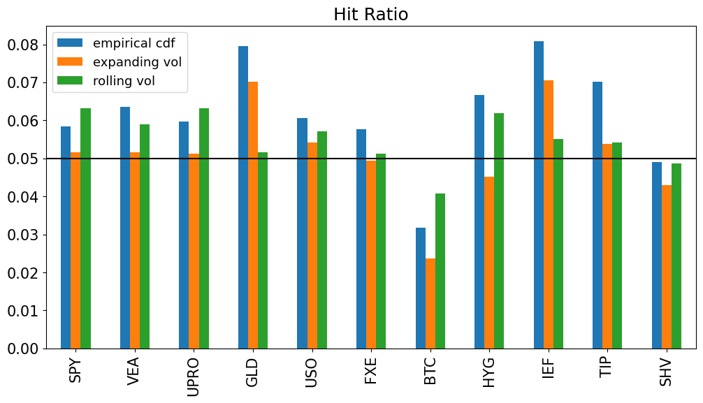
sum_sq_errors = ((hitratio-QUANTILE)**2).sum().to_frame('hit ratio errors')
sum_sq_errors.style.format('{:.2%}')

	hit ratio errors
empirical cdf	0.34%
expanding vol	0.16%
rolling vol	0.08%

tick = 'GLD'

fig, ax = plt.subplots(len(METHODS),1,figsize=(12,15))

for i,method in enumerate(METHODS):
    VaRret[method][tick].plot(ax=ax[i],title=f'{tick} VaR {method}')
    for xval in rets.index[hits.swaplevel(axis=1)[tick][method]]:
        ax[i].axvline(x=xval,color='lightgray', zorder=0)
    
plt.tight_layout()
plt.show()

Simulation

Historic Simulation (Empirical CDF)

Historical simulation is one of the simplest and most widely used approaches to calculating VaR.

• The historical simulation does not assume normally distributed losses.

• However, it is an unconditional VaR, in that it assumes independent observations.

• It takes the cdf of losses from the histogram of past losses.

Calculate the \(\VaR\) as the empirical quantile, exactly as discussed earlier.

CVaR

Obtain the \(\CVaR\) again using the order statistics to build the cdf:

\[r^{\CVaR_{\quant,1}} = \frac{1}{\quant\Ntime}\sum_{i=1}^{\quant\Ntime}r_{(i)}\]

This is just the sample mean of the left tail of the empirical cdf.

Advantages of Historical Simulation

Advantages of historical simulation This approach estimates a cdf of losses nonparametrically by assuming the subsample frequency reflects the actual probabilities.

• Thus, the estimated cdf can have any shape, based on the historic observations.

• The two main advantages here are the ease of implementation and the flexibility in not assuming a probability distribution, (such as the normal,) ex-ante.

Disadvantages of Historical Simulation

Statistical Power

The VaR depends on having a good estimate of the tail of the distribution.

• If the sample size, N, is small, then there will be large standard errors on the order statistic. (The standard errors shrink by the square root of the sample size.)

• If stress-testing extreme market conditions, need a sample of 10,000 just to get 10 observations in the 0.1% tail of the distribution.

Dynamics

The approach assumes returns are iid, which they are not.

• Take too big of a sample, and may be including irrelevant data, data which came from different distribution compared to data going forward.

• But too small a sample, and no precision.

Monte Carlo Simulation

Monte Carlo simulation generates data according to some statistical model.

1. Use each simulated observation to construct the corresponding portfolio loss.

2. Build an empirical cdf (histogram) from these simulated losses, and select the appropriate quantile.

MC has many applications:

• Historical approach simply skips the first step by taking observed past as the generated data.

• By using simulated cdf no need to worry about keeping the cdf tractable. Important for complicated dynamics or nonlinear valuation.

Simulating Bonds and Options

Monte Carlo simulation is usefully applied to cases where the portfolio value is nonlinear in the simulated factors.

• Consider simulating stock prices and then plugging the simulated data into Black-Scholes to obtain simulated losses on options.

• Simulate interest rates and then calculate bond portfolio losses as nonlinear function of these simulated data.

Other Approaches

\(t\)-distribution

The normal distribution was not good enough, so why not try other known distributions?

This is indeed done, most notably with the Student’s \(t\) distribution.

• Fatter tails than a normal, so will do better.

• But in some senses, it is a half-measure: computational work that is less useful for quoting and baseline, yet not enough computational work to be as serious as we would like.

Extreme Value Theory

Other distributions do not fit the center of the return data well.

Thus, Extreme Value Theory seeks distributions only for the extreme values of the distribution.

• Uses mathematical results to model just the tail.

Quantile Regression

Empically try to estimate the quantiles using some conditioning information, rather than the direct approach discussed above.