Factor VaR for a Long-Short Equity Book

The companion notebook simulates VaR for a handful of assets by fitting a GARCH to each one. That does not scale: a long-short equity book holds hundreds of names, and you cannot fit hundreds of stable volatility models.

The fix is a factor model. A few sector factors carry most of the co-movement (see LFD for Dimension Reduction), so we:

• regress each stock on the sectors to get its loadings and idiosyncratic return,

• fit GARCH to the sector factors only - a handful of models, not hundreds,

• run the filtered historical simulation through the factor structure.

The portfolio is a dollar-neutral momentum book: long recent winners, short recent losers. We work at daily frequency, so the backtest has enough observations to judge each method within a stress episode.

import pandas as pd
import numpy as np
import matplotlib.pyplot as plt
%matplotlib inline
plt.rcParams['figure.figsize'] = (10,5)
plt.rcParams['font.size'] = 13

import warnings
warnings.filterwarnings('ignore')
from arch import arch_model
from scipy.stats import norm

np.random.seed(2025)

stocks_all = pd.read_parquet('../data/spx_returns_daily_full.parquet')
sectors    = pd.read_excel('../data/sector_etf_data_daily.xlsx', sheet_name='total returns').set_index('date')

# align to dates where all sectors exist (XLC/XLRE start after 2015), then keep
# stocks with a full history over that window (a rectangular panel)
dates = stocks_all.index.intersection(sectors.index)
S = sectors.loc[dates].dropna()
R = stocks_all.loc[S.index].dropna(axis=1)
S = S.loc[R.index]

FREQ = 252
QUANTILE = 0.05
print(f'{R.shape[1]} stocks, {S.shape[1]} sector factors, daily, {R.index[0].date()} to {R.index[-1].date()}')

475 stocks, 11 sector factors, daily, 2018-06-20 to 2026-06-22

The Portfolio

Rank stocks by trailing twelve-month return (skipping the most recent month), go long the top quintile and short the bottom quintile, equal-weighted and dollar-neutral. These are today’s weights - the book we want the one-day VaR of.

mom = R.iloc[-273:-21].sum()                   # trailing 12-month return, skip last month
n_leg = len(mom)//5                            # quintiles
w = pd.Series(0.0, index=R.columns)
w[mom.nlargest(n_leg).index] =  1/n_leg        # long winners
w[mom.nsmallest(n_leg).index] = -1/n_leg       # short losers
print(f'long {n_leg}, short {n_leg}, gross {np.abs(w).sum():.0f}, net {w.sum():+.2f}')

long 95, short 95, gross 2, net +0.00

What the Book Holds

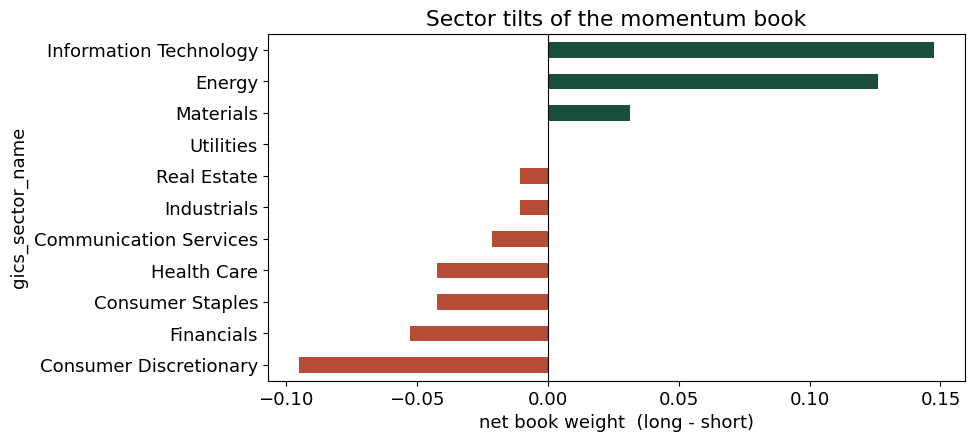
Two hundred equal-weighted positions is too many to list, but the story is in the tilts. Momentum is not sector-neutral: the winners and losers cluster in different sectors, so the dollar-neutral book still carries real sector bets - which is exactly the factor exposure the VaR must capture.

names = pd.read_excel('../data/spx_returns_weekly.xlsx', sheet_name='spx names').set_index('ticker')
name_of = names['name']
sector  = names['gics_sector_name'].reindex(w.index)

sec_w = w.groupby(sector).sum().sort_values()   # net sector weight (long minus short)

fig, ax = plt.subplots(figsize=(9,4.5))
sec_w.plot.barh(ax=ax, color=['#b64c33' if x < 0 else '#1b4d3e' for x in sec_w])
ax.axvline(0, color='black', lw=0.8)
ax.set_xlabel('net book weight  (long - short)')
ax.set_title('Sector tilts of the momentum book')
plt.show()

picks = pd.DataFrame({
    'top longs':  [name_of.get(t, t) for t in mom[w[w>0].index].nlargest(6).index],
    'top shorts': [name_of.get(t, t) for t in mom[w[w<0].index].nsmallest(6).index]})
picks.style.hide(axis='index').set_caption('Sharpest winners (long) and losers (short)')

Sharpest winners (long) and losers (short)

top longs	top shorts
Lumentum Holdings Inc	Trade Desk Inc/The
Western Digital Corp	Charter Communications Inc
SATS	Gartner Inc
Micron Technology Inc	Lululemon Athletica Inc
Seagate Technology Holdings PL	CoStar Group Inc
Ciena Corp	Workday Inc

Factor Structure

Regress each stock on the sector factors. Keep the loadings (systematic exposure) and the residual (idiosyncratic return).

X = np.column_stack([np.ones(len(S)), S.values])          # T x (1+k)
coef = np.linalg.lstsq(X, R.values, rcond=None)[0]        # (1+k) x n
alpha, B = coef[0], coef[1:]                              # alpha: n ,  B: k x n
resid = R.values - X @ coef                              # T x n idiosyncratic

r2 = 1 - resid.var(0)/R.values.var(0)
pd.Series(r2, index=R.columns).describe()[['mean','50%','min','max']].to_frame('stock R2 on sectors').style.format('{:.1%}').set_caption('How much of each stock the sectors explain')

How much of each stock the sectors explain

	stock R2 on sectors
mean	50.3%
50%	49.5%
min	9.0%
max	86.8%

GARCH on the Sector Factors

Fit a GARCH(1,1) to each sector factor - eleven models, regardless of how many stocks the book holds. Keep the standardized shocks, the conditional-volatility series, and the current level.

k = S.shape[1]
Zf  = np.empty((len(S), k))       # standardized factor shocks
CVf = np.empty((len(S), k))       # conditional vol series

for j, s in enumerate(S.columns):
    res = arch_model(S[s]*100, mean='Constant', vol='GARCH', p=1, q=1).fit(disp='off')
    Zf[:, j]  = res.std_resid
    CVf[:, j] = res.conditional_volatility / 100

sig_now = CVf[-1]                  # current (latest) conditional volatility
(pd.Series(sig_now*np.sqrt(FREQ), index=S.columns).sort_values(ascending=False)
 .to_frame('ann. vol, current').style.format('{:.1%}').set_caption('Current sector-factor volatility'))

Current sector-factor volatility

	ann. vol, current
XLK	40.7%
XLE	27.3%
XLY	24.6%
XLB	22.0%
XLI	21.0%
XLC	19.9%
XLRE	19.4%
XLF	16.9%
XLU	16.8%
XLP	16.5%
XLV	16.3%

Filtered Historical Simulation

Draw a historical day. Take that day’s standardized factor shocks (re-inflated to the current factor volatility) and its idiosyncratic residuals - both from the same day, so the cross-sectional structure survives. Rebuild each stock as loadings times factors plus idiosyncratic, then form the book.

M = 50_000
idx = np.random.randint(0, len(Zf), size=M)

factor_sim = Zf[idx] * sig_now                  # M x k, at the current volatility
stock_sim  = alpha + factor_sim @ B + resid[idx]   # M x n
port_sim   = stock_sim @ w.values               # M book returns

cut = np.quantile(port_sim, QUANTILE)
print(f'Factor-FHS  VaR(5%) = {-cut:.2%}    CVaR(5%) = {-port_sim[port_sim<=cut].mean():.2%}')

Factor-FHS  VaR(5%) = 1.47%    CVaR(5%) = 2.20%

VaR Through Time

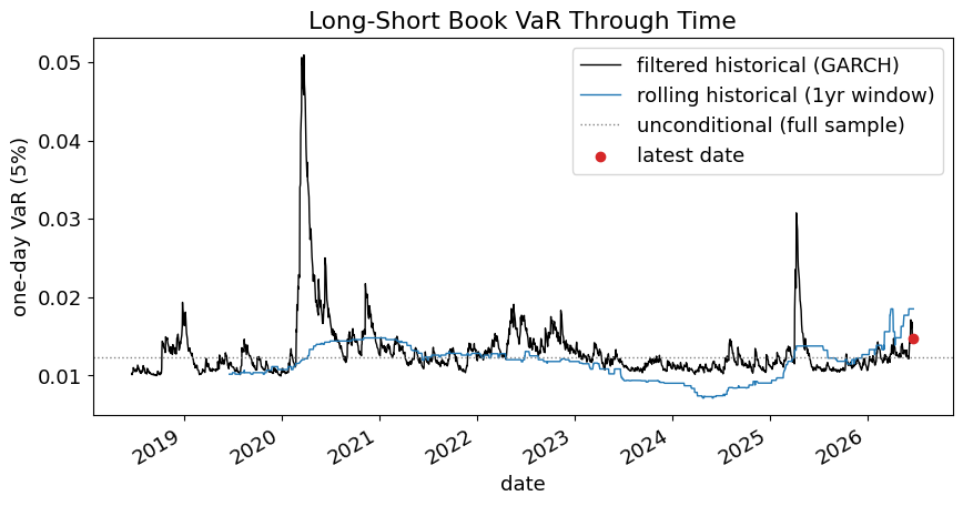
Re-evaluate the book’s one-day VaR at every date, and compare like with like: a rolling historical VaR (a one-year window, recomputed daily) also conditions on the regime, so this is a fair test.

The GARCH-filtered VaR reacts within days; the rolling window lags - a shock takes a year to enter the window and then lingers for a year before dropping out as a cliff. The full-sample line is only an anchor.

bw  = B @ w.values                 # book's factor exposure
rw  = resid @ w.values             # book's idiosyncratic return series
const = float(w.values @ alpha)
rp  = pd.Series(R.values @ w.values, index=R.index)   # book's realized daily returns

WIN = 252                                             # one-year rolling window
roll_hist  = -rp.rolling(WIN).quantile(QUANTILE)      # conditional historical, recomputed daily
var_uncond = -rp.quantile(QUANTILE)                   # full-sample anchor
fhs_t = pd.Series([-(const + np.quantile(Zf @ (bw * CVf[i]) + rw, QUANTILE)) for i in range(len(R))],
                  index=R.index)

fig, ax = plt.subplots()
fhs_t.plot(ax=ax, color='black', lw=1.0, label='filtered historical (GARCH)')
roll_hist.plot(ax=ax, color='C0', lw=1.0, label='rolling historical (1yr window)')
ax.axhline(var_uncond, color='gray', ls=':', lw=1, label='unconditional (full sample)')
ax.scatter([R.index[-1]], [fhs_t.iloc[-1]], color='C3', zorder=5, label='latest date')
ax.set_ylabel('one-day VaR (5%)')
ax.set_title('Long-Short Book VaR Through Time')
ax.legend()
plt.show()

Backtesting: How Often Is VaR Breached?

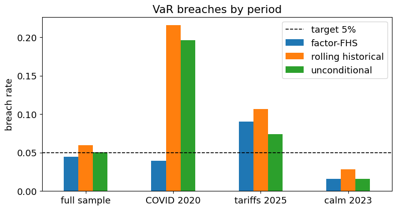
A 5% VaR should be breached about 5% of days - no more, and not bunched up. The full-sample rate flatters every method; the regime split is where they separate. A method that ignores the volatility regime over-breaches in stress, so by arithmetic it must under-breach elsewhere - over-conservative right after a crash, then caught short by the next one.

methods = {'factor-FHS':          fhs_t,
           'rolling historical':  roll_hist,
           'unconditional':       pd.Series(var_uncond, index=R.index)}
periods = {'full sample':  slice(None),
           'COVID 2020':   slice('2020-02-19', '2020-04-30'),
           'tariffs 2025': slice('2025-01-01', '2025-06-30'),
           'calm 2023':    slice('2023-01-01', '2023-12-31')}

def hit_rate(var, sl):
    breach = (rp < -var.shift(1))[var.shift(1).notna()]
    return breach.loc[sl].mean()

hits = pd.DataFrame({m: {p: hit_rate(v, sl) for p, sl in periods.items()} for m, v in methods.items()}).T
display(hits.style.format('{:.1%}').background_gradient(cmap='Reds', vmin=0.05, vmax=0.30)
        .set_caption('Share of days the next return breached the 5% VaR (target 5%)'))

ax = hits.T.plot.bar(figsize=(9,4.5), rot=0)
ax.axhline(0.05, color='black', ls='--', lw=1.2, label='target 5%')
ax.set_ylabel('breach rate'); ax.set_title('VaR breaches by period'); ax.legend()
plt.show()

Share of days the next return breached the 5% VaR (target 5%)

	full sample	COVID 2020	tariffs 2025	calm 2023
factor-FHS	4.5%	3.9%	9.0%	1.6%
rolling historical	6.0%	21.6%	10.7%	2.8%
unconditional	5.0%	19.6%	7.4%	1.6%

Notes

• Where the factor model earns its keep. We fit GARCH to eleven sector factors, not to hundreds of stocks. The idiosyncratic piece is left homoskedastic and simply resampled - cheap and stable.

• Long-short and factor risk. A dollar-neutral book still carries factor exposure B'w; if the long and short legs load differently on sectors, the book’s VaR is driven by those factor bets.

• The idiosyncratic caveat. Momentum crashes are partly idiosyncratic - the winners and losers reverse against each other, not just with the sectors. A homoskedastic idiosyncratic term will understate the book’s tail in exactly those episodes, which the backtest can reveal.