Mexican Peso Crisis 1994

Mexican Peso Crisis 1994#

The Peso Problem#

The Mexican peso crisis of December 1994 provides a classic example of carry trade risk. Throughout 1994, the Mexican peso offered attractive interest rates relative to the US dollar, making it a popular carry trade target. However, the peso’s unexpected 50%+ devaluation in late December 1994 wiped out years of carry profits in a matter of days.

This crisis illustrates the fundamental risk in carry trades: the carry component is typically small and steady, while the FX component can be large and sudden.

import pandas as pd
import numpy as np
import matplotlib.pyplot as plt
from datetime import datetime
import pandas_datareader.data as web

%matplotlib inline
plt.rcParams['figure.figsize'] = (12,6)
plt.rcParams['font.size'] = 13
plt.rcParams['legend.fontsize'] = 13

from cmds.portfolio import performanceMetrics, tailMetrics

Data Collection#

We collect three key series from FRED:

IRSTCI01MXM156N: Mexican interest rate (1-month, % annual)
FEDFUNDS: US Federal Funds rate (% annual)
EXMXUS: MXN/USD exchange rate (Mexican pesos per US dollar)

The analysis covers 1993-1996 to capture the pre-crisis buildup and post-crisis aftermath.

# Data collection from FRED
start_date = '1993-01-01'
end_date = '1996-12-31'

# Mexican interest rate (1-month, % annual)
mx_rate = web.DataReader('IRSTCI01MXM156N', 'fred', start_date, end_date)
mx_rate.columns = ['MX_RATE']

# US Federal Funds rate (% annual)
us_rate = web.DataReader('FEDFUNDS', 'fred', start_date, end_date)
us_rate.columns = ['US_RATE']

# Exchange rate: MXN per USD
fx_rate = web.DataReader('EXMXUS', 'fred', start_date, end_date)
fx_rate.columns = ['MXN_USD']

print(f"Data coverage:")
print(f"Mexican rate: {mx_rate.index[0].strftime('%Y-%m-%d')} to {mx_rate.index[-1].strftime('%Y-%m-%d')}")
print(f"US rate: {us_rate.index[0].strftime('%Y-%m-%d')} to {us_rate.index[-1].strftime('%Y-%m-%d')}")
print(f"FX rate: {fx_rate.index[0].strftime('%Y-%m-%d')} to {fx_rate.index[-1].strftime('%Y-%m-%d')}")

Data coverage:
Mexican rate: 1993-01-01 to 1996-12-01
US rate: 1993-01-01 to 1996-12-01
FX rate: 1993-11-01 to 1996-12-01

# Combine data and handle missing values
data = pd.concat([mx_rate, us_rate, fx_rate], axis=1)
data = data.dropna()

# Convert annual rates to monthly (approximately)
data['MX_RATE_MONTHLY'] = data['MX_RATE'] / 12 / 100  # Convert % annual to decimal monthly
data['US_RATE_MONTHLY'] = data['US_RATE'] / 12 / 100  # Convert % annual to decimal monthly

# Calculate monthly FX returns (MXN appreciation/depreciation)
data['FX_RETURN'] = data['MXN_USD'].pct_change()

print(f"Sample period: {data.index[0].strftime('%Y-%m-%d')} to {data.index[-1].strftime('%Y-%m-%d')}")
display(data.head().style.format('{:.2f}'))

Sample period: 1993-11-01 to 1996-12-01

	MX_RATE	US_RATE	MXN_USD	MX_RATE_MONTHLY	US_RATE_MONTHLY	FX_RETURN
DATE
1993-11-01 00:00:00	16.62	3.02	3.15	0.01	0.00	nan
1993-12-01 00:00:00	14.68	2.96	3.11	0.01	0.00	-0.01
1994-01-01 00:00:00	13.22	3.05	3.11	0.01	0.00	-0.00
1994-02-01 00:00:00	11.96	3.25	3.12	0.01	0.00	0.00
1994-03-01 00:00:00	11.53	3.34	3.30	0.01	0.00	0.06

Visualizing the Crisis Setup#

fig, ((ax1, ax2), (ax3, ax4)) = plt.subplots(2, 2, figsize=(15, 10))

# Interest rate differential
rate_diff = data['MX_RATE'] - data['US_RATE']
ax1.plot(data.index, rate_diff, 'b-', linewidth=2)
ax1.axvline(datetime(1994, 12, 20), color='red', linestyle='--', alpha=0.7, label='Peso Devaluation')
ax1.set_title('Interest Rate Differential\n(Mexican Rate - US Fed Funds)', fontweight='bold')
ax1.set_ylabel('Rate Differential (%)')
ax1.grid(True, alpha=0.3)
ax1.legend()

# Exchange rate
ax2.plot(data.index, data['MXN_USD'], 'g-', linewidth=2)
ax2.axvline(datetime(1994, 12, 20), color='red', linestyle='--', alpha=0.7, label='Peso Devaluation')
ax2.set_title('MXN/USD Exchange Rate\n(Pesos per Dollar)', fontweight='bold')
ax2.set_ylabel('MXN per USD')
ax2.grid(True, alpha=0.3)
ax2.legend()

# Individual rates
ax3.plot(data.index, data['MX_RATE'], 'r-', linewidth=2, label='Mexican Rate')
ax3.plot(data.index, data['US_RATE'], 'b-', linewidth=2, label='US Fed Funds')
ax3.axvline(datetime(1994, 12, 20), color='red', linestyle='--', alpha=0.7)
ax3.set_title('Interest Rates', fontweight='bold')
ax3.set_ylabel('Interest Rate (%)')
ax3.legend()
ax3.grid(True, alpha=0.3)

# FX monthly returns
ax4.plot(data.index[1:], data['FX_RETURN'][1:]*100, 'purple', linewidth=1)
ax4.axvline(datetime(1994, 12, 20), color='red', linestyle='--', alpha=0.7, label='Peso Devaluation')
ax4.axhline(0, color='black', linestyle='-', alpha=0.3)
ax4.set_title('Monthly FX Returns\n(Positive = Peso Weakening)', fontweight='bold')
ax4.set_ylabel('FX Return (%)')
ax4.legend()
ax4.grid(True, alpha=0.3)

plt.tight_layout()
plt.show()

# Key statistics around the crisis
crisis_month = datetime(1994, 12, 1)
crisis_fx_return = data.loc[data.index >= crisis_month, 'FX_RETURN'].iloc[0] if len(data.loc[data.index >= crisis_month]) > 0 else np.nan

print(f"\nCrisis Statistics:")
if not np.isnan(crisis_fx_return):
    print(f"December 1994 FX return: {crisis_fx_return*100:.1f}% (peso weakening)")
print(f"Pre-crisis average rate differential (1994): {rate_diff['1994'].mean():.1f}%")
print(f"Exchange rate: {data.loc['1994-01', 'MXN_USD'].iloc[0]:.2f} (Jan 1994) → {data.loc['1995-01', 'MXN_USD'].iloc[0]:.2f} (Jan 1995)")

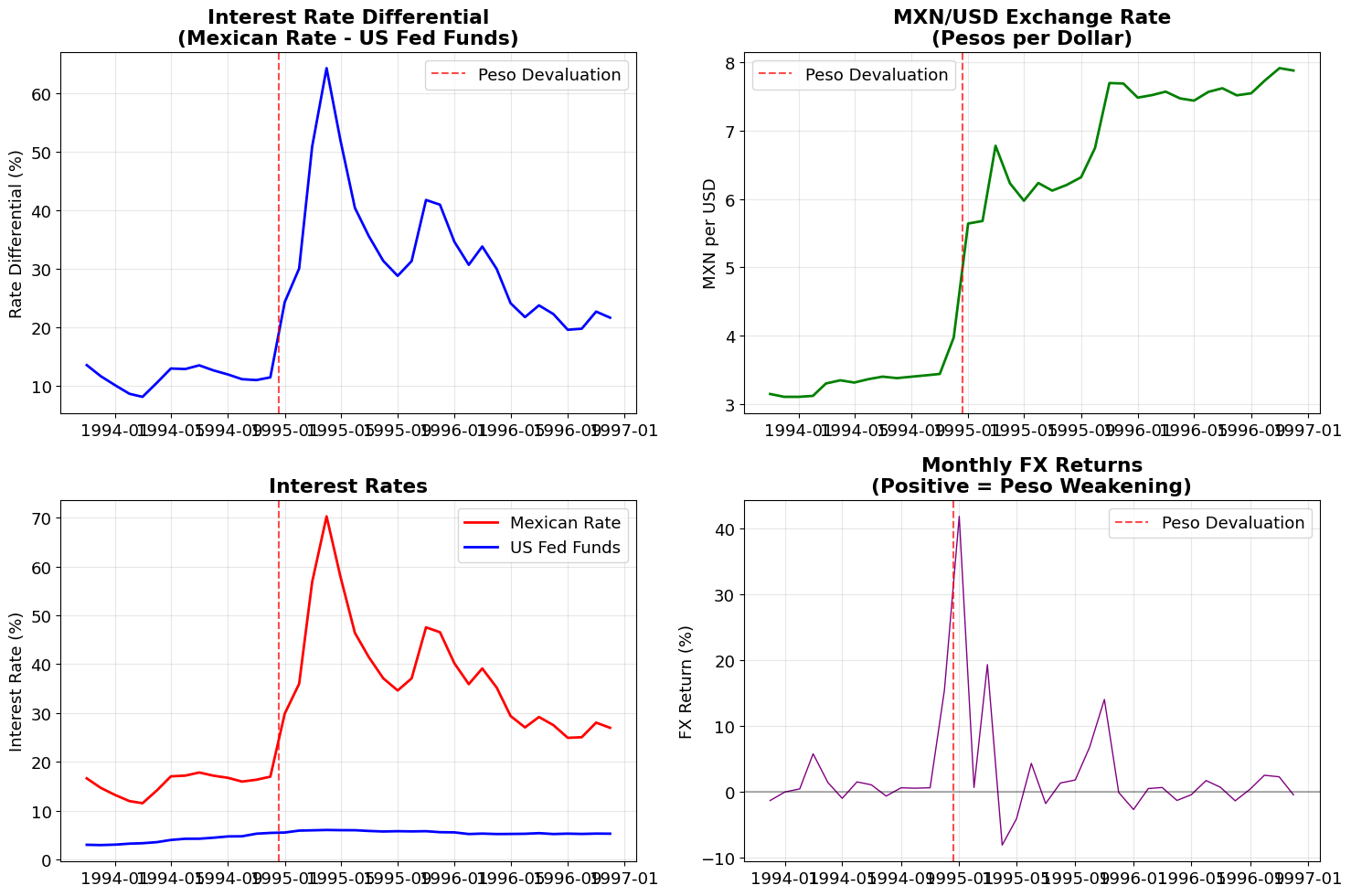
../_images/965d33f9f0d0a0382b5f2bcbfd44db11e952ad8b4212bee3fc295000dfced19f.png

Crisis Statistics:
December 1994 FX return: 15.5% (peso weakening)
Pre-crisis average rate differential (1994): 11.3%
Exchange rate: 3.11 (Jan 1994) → 5.64 (Jan 1995)

Building the Carry Trade#

The carry trade strategy:

Borrow in the low-yield currency (USD)
Invest in the high-yield currency (MXN)
Currency risk: Exposed to MXN/USD exchange rate changes

Monthly return decomposition:

Carry component: Interest rate differential earned
FX component: Currency appreciation/depreciation
Total return: Carry + FX components

# Calculate carry trade returns
# Carry component: Interest rate differential (what we earn from rate difference)
data['CARRY_RETURN'] = data['MX_RATE_MONTHLY'] - data['US_RATE_MONTHLY']

# FX component: Currency moves (negative because MXN weakening hurts our position)
# When MXN_USD increases, peso weakens, which hurts our peso position
data['FX_COMPONENT'] = -data['FX_RETURN']

# Total return: Carry + FX components
data['TOTAL_RETURN'] = data['CARRY_RETURN'] + data['FX_COMPONENT']

# Calculate cumulative returns
data['CUM_CARRY'] = (1 + data['CARRY_RETURN']).cumprod() - 1
data['CUM_FX'] = (1 + data['FX_COMPONENT']).cumprod() - 1  
data['CUM_TOTAL'] = (1 + data['TOTAL_RETURN']).cumprod() - 1

print("Carry Trade Return Components:")
print(f"Average monthly carry: {data['CARRY_RETURN'].mean()*100:.2f}%")
print(f"Average monthly FX impact: {data['FX_COMPONENT'].mean()*100:.2f}%")
print(f"Average monthly total: {data['TOTAL_RETURN'].mean()*100:.2f}%")
print(f"\nVolatility (monthly):")
print(f"Carry volatility: {data['CARRY_RETURN'].std()*100:.2f}%")
print(f"FX volatility: {data['FX_COMPONENT'].std()*100:.2f}%")
print(f"Total volatility: {data['TOTAL_RETURN'].std()*100:.2f}%")

Carry Trade Return Components:
Average monthly carry: 2.06%
Average monthly FX impact: -2.79%
Average monthly total: -0.71%

Volatility (monthly):
Carry volatility: 1.13%
FX volatility: 8.34%
Total volatility: 8.42%

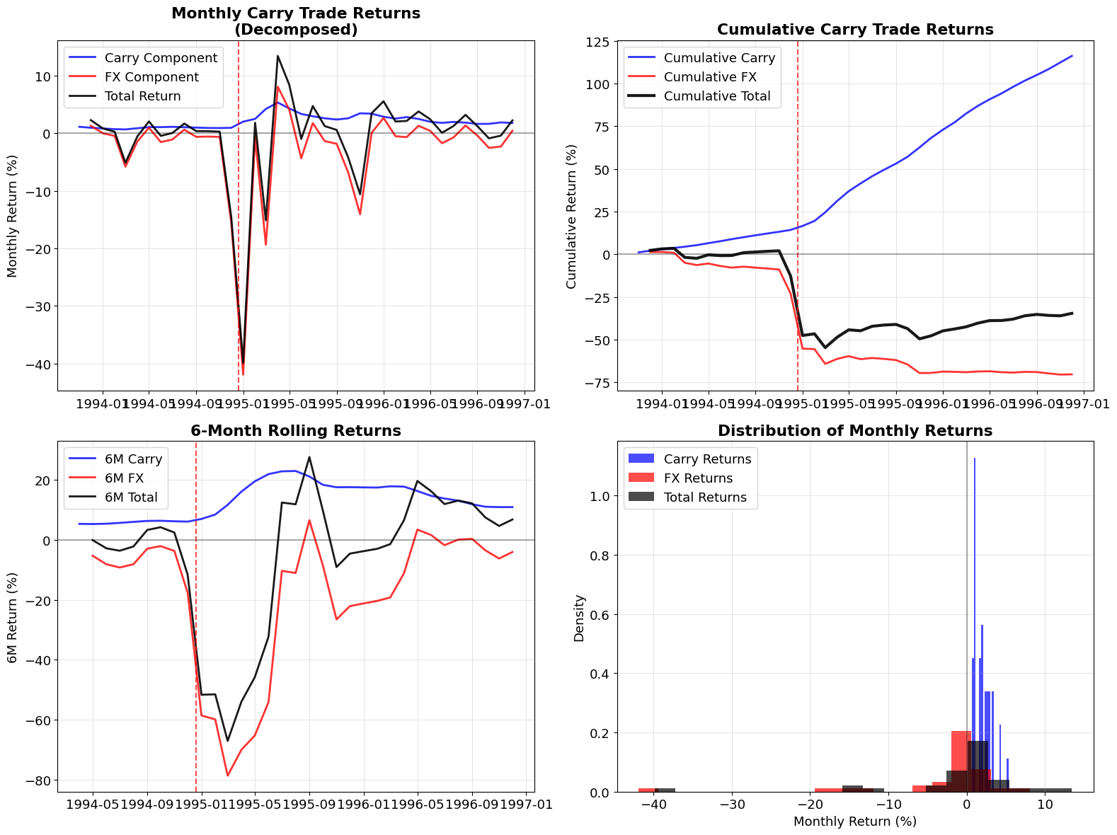
Return Decomposition Analysis#

fig, ((ax1, ax2), (ax3, ax4)) = plt.subplots(2, 2, figsize=(16, 12))

# Monthly returns decomposition
ax1.plot(data.index, data['CARRY_RETURN']*100, 'b-', linewidth=2, label='Carry Component', alpha=0.8)
ax1.plot(data.index, data['FX_COMPONENT']*100, 'r-', linewidth=2, label='FX Component', alpha=0.8)
ax1.plot(data.index, data['TOTAL_RETURN']*100, 'k-', linewidth=2, label='Total Return', alpha=0.9)
ax1.axvline(datetime(1994, 12, 20), color='red', linestyle='--', alpha=0.7)
ax1.axhline(0, color='black', linestyle='-', alpha=0.3)
ax1.set_title('Monthly Carry Trade Returns\n(Decomposed)', fontweight='bold')
ax1.set_ylabel('Monthly Return (%)')
ax1.legend()
ax1.grid(True, alpha=0.3)

# Cumulative returns
ax2.plot(data.index, data['CUM_CARRY']*100, 'b-', linewidth=2, label='Cumulative Carry', alpha=0.8)
ax2.plot(data.index, data['CUM_FX']*100, 'r-', linewidth=2, label='Cumulative FX', alpha=0.8)
ax2.plot(data.index, data['CUM_TOTAL']*100, 'k-', linewidth=3, label='Cumulative Total', alpha=0.9)
ax2.axvline(datetime(1994, 12, 20), color='red', linestyle='--', alpha=0.7)
ax2.axhline(0, color='black', linestyle='-', alpha=0.3)
ax2.set_title('Cumulative Carry Trade Returns', fontweight='bold')
ax2.set_ylabel('Cumulative Return (%)')
ax2.legend()
ax2.grid(True, alpha=0.3)

# Rolling 6-month performance
rolling_window = 6
rolling_carry = data['CARRY_RETURN'].rolling(window=rolling_window).sum()*100
rolling_fx = data['FX_COMPONENT'].rolling(window=rolling_window).sum()*100
rolling_total = data['TOTAL_RETURN'].rolling(window=rolling_window).sum()*100

ax3.plot(data.index, rolling_carry, 'b-', linewidth=2, label=f'{rolling_window}M Carry', alpha=0.8)
ax3.plot(data.index, rolling_fx, 'r-', linewidth=2, label=f'{rolling_window}M FX', alpha=0.8)
ax3.plot(data.index, rolling_total, 'k-', linewidth=2, label=f'{rolling_window}M Total', alpha=0.9)
ax3.axvline(datetime(1994, 12, 20), color='red', linestyle='--', alpha=0.7)
ax3.axhline(0, color='black', linestyle='-', alpha=0.3)
ax3.set_title(f'{rolling_window}-Month Rolling Returns', fontweight='bold')
ax3.set_ylabel('6M Return (%)')
ax3.legend()
ax3.grid(True, alpha=0.3)

# Distribution of monthly returns
ax4.hist(data['CARRY_RETURN']*100, bins=20, alpha=0.7, label='Carry Returns', density=True, color='blue')
ax4.hist(data['FX_COMPONENT']*100, bins=20, alpha=0.7, label='FX Returns', density=True, color='red')
ax4.hist(data['TOTAL_RETURN']*100, bins=20, alpha=0.7, label='Total Returns', density=True, color='black')
ax4.axvline(0, color='black', linestyle='-', alpha=0.3)
ax4.set_title('Distribution of Monthly Returns', fontweight='bold')
ax4.set_xlabel('Monthly Return (%)')
ax4.set_ylabel('Density')
ax4.legend()
ax4.grid(True, alpha=0.3)

plt.tight_layout()
plt.show()

../_images/15e9df69a11a312b85df8381cc760d84edb7202a149c153d9dedb2a6a0cf4770.png

Crisis Impact Analysis#

# Analyze the crisis period in detail
crisis_start = datetime(1994, 12, 1)
crisis_end = datetime(1995, 3, 31)

pre_crisis = data[data.index < crisis_start].copy()
crisis_period = data[(data.index >= crisis_start) & (data.index <= crisis_end)].copy()
post_crisis = data[data.index > crisis_end].copy()

print("=" * 60)
print("MEXICAN PESO CARRY TRADE CRISIS ANALYSIS")
print("=" * 60)

print(f"\nPRE-CRISIS PERIOD (Through Nov 1994):")
print(f"  Months: {len(pre_crisis)}")
print(f"  Cumulative carry earned: {pre_crisis['CUM_CARRY'].iloc[-1]*100:.1f}%")
print(f"  Cumulative FX impact: {pre_crisis['CUM_FX'].iloc[-1]*100:.1f}%")
print(f"  Cumulative total return: {pre_crisis['CUM_TOTAL'].iloc[-1]*100:.1f}%")
print(f"  Average monthly carry: {pre_crisis['CARRY_RETURN'].mean()*100:.2f}%")
print(f"  FX volatility: {pre_crisis['FX_COMPONENT'].std()*100:.2f}%")

print(f"\nCRISIS PERIOD (Dec 1994 - Mar 1995):")
print(f"  Months: {len(crisis_period)}")
if len(crisis_period) > 0:
    print(f"  Crisis period carry: {crisis_period['CARRY_RETURN'].sum()*100:.1f}%")
    print(f"  Crisis period FX impact: {crisis_period['FX_COMPONENT'].sum()*100:.1f}%")
    print(f"  Crisis period total: {crisis_period['TOTAL_RETURN'].sum()*100:.1f}%")
    print(f"  Worst monthly FX loss: {crisis_period['FX_COMPONENT'].min()*100:.1f}%")
    print(f"  Worst monthly total loss: {crisis_period['TOTAL_RETURN'].min()*100:.1f}%")

print(f"\nPOST-CRISIS PERIOD (Apr 1995 onwards):")
print(f"  Months: {len(post_crisis)}")
if len(post_crisis) > 0:
    post_crisis_total_from_start = (1 + post_crisis['TOTAL_RETURN']).cumprod().iloc[-1] - 1
    print(f"  Recovery total return: {post_crisis_total_from_start*100:.1f}%")
    print(f"  Average monthly carry: {post_crisis['CARRY_RETURN'].mean()*100:.2f}%")

print(f"\nOVERALL STRATEGY PERFORMANCE:")
final_carry = data['CUM_CARRY'].iloc[-1]*100
final_fx = data['CUM_FX'].iloc[-1]*100 
final_total = data['CUM_TOTAL'].iloc[-1]*100
print(f"  Total cumulative carry: {final_carry:.1f}%")
print(f"  Total cumulative FX: {final_fx:.1f}%")
print(f"  Total cumulative return: {final_total:.1f}%")

# Risk metrics
total_returns_monthly = data['TOTAL_RETURN'].dropna()
if len(total_returns_monthly) > 0:
    annual_return = (1 + total_returns_monthly.mean())**12 - 1
    annual_vol = total_returns_monthly.std() * np.sqrt(12)
    sharpe = annual_return / annual_vol if annual_vol > 0 else 0
    max_drawdown = ((1 + data['TOTAL_RETURN']).cumprod() / (1 + data['TOTAL_RETURN']).cumprod().cummax() - 1).min()
    
    print(f"\nRISK METRICS:")
    print(f"  Annualized return: {annual_return*100:.1f}%")
    print(f"  Annualized volatility: {annual_vol*100:.1f}%")
    print(f"  Sharpe ratio: {sharpe:.2f}")
    print(f"  Maximum drawdown: {max_drawdown*100:.1f}%")

============================================================
MEXICAN PESO CARRY TRADE CRISIS ANALYSIS
============================================================

PRE-CRISIS PERIOD (Through Nov 1994):
  Months: 13
  Cumulative carry earned: 13.2%
  Cumulative FX impact: -8.9%
  Cumulative total return: 2.0%
  Average monthly carry: 0.96%
  FX volatility: 1.82%

CRISIS PERIOD (Dec 1994 - Mar 1995):
  Months: 4
  Crisis period carry: 9.7%
  Crisis period FX impact: -77.4%
  Crisis period total: -67.7%
  Worst monthly FX loss: -41.9%
  Worst monthly total loss: -39.9%

POST-CRISIS PERIOD (Apr 1995 onwards):
  Months: 21
  Recovery total return: 44.2%
  Average monthly carry: 2.66%

OVERALL STRATEGY PERFORMANCE:
  Total cumulative carry: 116.2%
  Total cumulative FX: -70.3%
  Total cumulative return: -34.6%

RISK METRICS:
  Annualized return: -8.2%
  Annualized volatility: 29.2%
  Sharpe ratio: -0.28
  Maximum drawdown: -56.2%

Key Lessons from the Peso Crisis#

# Calculate some key ratios to illustrate the lesson
avg_monthly_carry = data['CARRY_RETURN'].mean() * 100
worst_monthly_fx = data['FX_COMPONENT'].min() * 100
fx_vol = data['FX_COMPONENT'].std() * 100
carry_vol = data['CARRY_RETURN'].std() * 100

print("KEY INSIGHTS FROM THE PESO CRISIS:")
print("="*50)
print(f"\n1. ASYMMETRIC RISK PROFILE:")
print(f"   • Average monthly carry pickup: +{avg_monthly_carry:.2f}%")
print(f"   • Worst monthly FX loss: {worst_monthly_fx:.1f}%")
print(f"   • Risk-return asymmetry: {abs(worst_monthly_fx/avg_monthly_carry):.0f}:1")

print(f"\n2. VOLATILITY SOURCES:")
print(f"   • Carry component volatility: {carry_vol:.2f}%")
print(f"   • FX component volatility: {fx_vol:.2f}%")
print(f"   • FX risk dominates: {fx_vol/carry_vol:.0f}x higher")

print(f"\n3. TIME TO RECOVER:")
# Find when strategy recovers to pre-crisis peak
pre_crisis_peak = data.loc[data.index < crisis_start, 'CUM_TOTAL'].max()
recovery_data = data.loc[data.index >= crisis_start, 'CUM_TOTAL']
recovery_point = recovery_data[recovery_data >= pre_crisis_peak]

if len(recovery_point) > 0:
    recovery_date = recovery_point.index[0]
    months_to_recover = (recovery_date - crisis_start).days / 30.44
    print(f"   • Crisis began: {crisis_start.strftime('%b %Y')}")
    print(f"   • Strategy recovered: {recovery_date.strftime('%b %Y')}")
    print(f"   • Time to recovery: {months_to_recover:.1f} months")
else:
    print(f"   • Strategy never fully recovered during sample period")

print(f"\n4. CRISIS CHARACTERISTICS:")
print(f"   • Build-up period: Steady carry profits with low FX volatility")
print(f"   • Crisis trigger: Political/economic instability")
print(f"   • Crisis impact: Sudden, large FX move overwhelms carry")
print(f"   • Classic 'peso problem': Small probability, large impact event")

KEY INSIGHTS FROM THE PESO CRISIS:
==================================================

1. ASYMMETRIC RISK PROFILE:
   • Average monthly carry pickup: +2.06%
   • Worst monthly FX loss: -41.9%
   • Risk-return asymmetry: 20:1

2. VOLATILITY SOURCES:
   • Carry component volatility: 1.13%
   • FX component volatility: 8.34%
   • FX risk dominates: 7x higher

3. TIME TO RECOVER:
   • Strategy never fully recovered during sample period

4. CRISIS CHARACTERISTICS:
   • Build-up period: Steady carry profits with low FX volatility
   • Crisis trigger: Political/economic instability
   • Crisis impact: Sudden, large FX move overwhelms carry
   • Classic 'peso problem': Small probability, large impact event

Summary#

The Mexican peso crisis of 1994 demonstrates the fundamental risk in carry trades:

The Carry Trade Paradox:

Carry component: Small, steady, predictable
FX component: Large, volatile, unpredictable
Result: Years of carry profits can be wiped out in days

Key Risk Factors:

Asymmetric payoffs: Limited upside from carry, unlimited downside from FX
Volatility mismatch: FX volatility dominates carry stability
Timing risk: Crisis events are unpredictable and sudden
Recovery time: Long periods needed to recover from crisis losses

This case study illustrates why carry trades are often described as “picking up pennies in front of a steamroller” - the strategy collects small, regular profits most of the time, but faces the risk of large, sudden losses that can more than offset years of gains.

Mexican Peso Crisis 1994

Contents

Mexican Peso Crisis 1994#

Mexican Peso Crisis 1994#

The Peso Problem#

Data Collection#

Visualizing the Crisis Setup#

Building the Carry Trade#

Return Decomposition Analysis#

Crisis Impact Analysis#

Key Lessons from the Peso Crisis#

Summary#