Equity Indexes and ETFs#
import pandas as pd
import numpy as np
import datetime
import warnings

from sklearn.linear_model import LinearRegression
from sklearn.decomposition import PCA
from scipy.optimize import minimize

import matplotlib.pyplot as plt
%matplotlib inline
plt.rcParams['figure.figsize'] = (12,6)
plt.rcParams['font.size'] = 15
plt.rcParams['legend.fontsize'] = 13

from matplotlib.ticker import (MultipleLocator,
                               FormatStrFormatter,
                               AutoMinorLocator)

import seaborn as sns

import sys
sys.path.insert(0, '..')
from utils import *
from portfolio import *
Indexes#
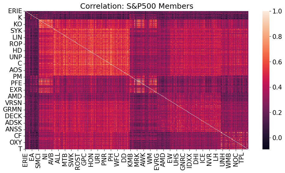
The S&P 500#
Constituents#
The S&P 500 is composed of
US-listed public equities
Large market cap
Liquid shares
A few extra conditions on financials to try to eliminate excess turnover
For practical purposes, consider it as the largest 500 U.S. equities.
Reference: S&P Index methodology, pgs 6-10
import scipy.cluster.hierarchy as sch

def cluster_corr(corr_array, inplace=False):
    """
    Rearranges the correlation matrix, corr_array, so that groups of highly
    correlated variables are next to eachother

    Parameters
    ----------
    corr_array : pandas.DataFrame or numpy.ndarray
        a NxN correlation matrix

    Returns
    -------
    pandas.DataFrame or numpy.ndarray
        a NxN correlation matrix with the columns and rows rearranged
    """
    pairwise_distances = sch.distance.pdist(corr_array)
    linkage = sch.linkage(pairwise_distances, method='complete')
    cluster_distance_threshold = pairwise_distances.max()/2
    idx_to_cluster_array = sch.fcluster(linkage, cluster_distance_threshold,
                                        criterion='distance')
    idx = np.argsort(idx_to_cluster_array)

    if not inplace:
        corr_array = corr_array.copy()

    if isinstance(corr_array, pd.DataFrame):
        return corr_array.iloc[idx, :].T.iloc[idx, :]
    return corr_array[idx, :][:, idx]
ALTFILE = "../data/spx_returns_weekly.xlsx"
FREQ = 52
rets_spx = pd.read_excel(ALTFILE, sheet_name="s&p500 rets").set_index("date")

sns.heatmap(cluster_corr(rets_spx.corr()))
plt.title('Correlation: S&P500 Members')
plt.show()
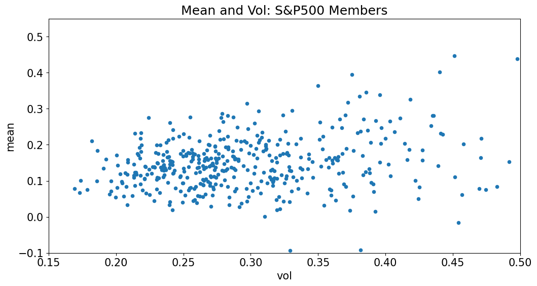
temp = pd.concat([rets_spx.mean()*FREQ, rets_spx.std()*FREQ**.5],axis=1)
temp.columns=['mean','vol']
temp.plot.scatter(x='vol',y='mean',xlim=(.15,.5),ylim=(-.1,.55));
plt.title('Mean and Vol: S&P500 Members');
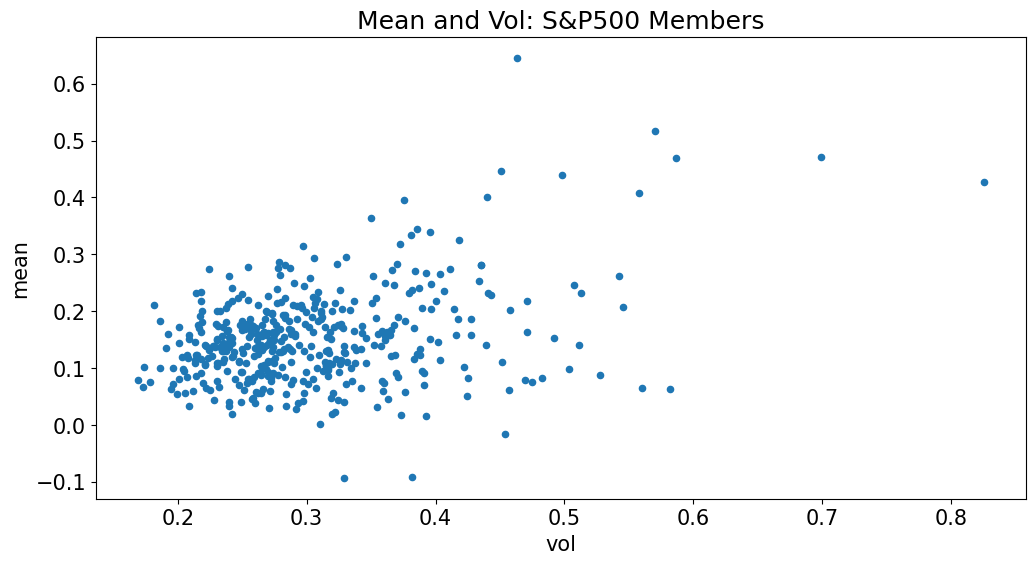
There is an outlier over this period#
The outlier is ENPH
joined the S&P 500 at the end of 2020
energy firm
volatile and high-trending returns
temp.plot.scatter(x='vol',y='mean');
plt.title('Mean and Vol: S&P500 Members');
Additional U.S. Equity Indexes#
Other U.S. equity indexes include many from the S&P:
S&P 100 - mega cap
S&P 1500 - large and medium cap
S&P Sector Indexes
Also consider
Russell 1000
Russell 2000
Wilshire 5000
Dow Jones Industrial#
In financial news, you will often see reference to the Dow Jones Industrial Average (DJIA)
You will rarely (if ever) use this
Prominent for historical reasons, but not a good choice for most applications/analysis
Problems with using it include
Index of only 30 “prominent” equities.
Weighting is by price, not by market cap.
Turnover may be too slow.
The DJIA is highly correlated to the S&P500, which is probably the only info of use to us in the index.
Exchange-based Indexes#
An important set of indexes are those that include stocks trading on a particular exchange.
NYSE Composite (New York)
NASDAQ Composite (New York)
FTSE 100 (London)
Nikkei 225 (Tokyo)
DAX (German)
Hang Seng (Hong Kong)
Additional International Equity Indexes#
MSCI indexes provide a wide number of indexes based on global regions and other global designations.
Style Indexes#
There are numerous style indexes used as benchmarks for various types of equity trading strategies.
By far, these indexes focus on
small vs large (size)
value vs growth (style)
Fama-French Factors#
The Fama-French Factors serve as popular indexes for these styles.
Particularly for historical research
Source: https://mba.tuck.dartmouth.edu/pages/faculty/ken.french/data_library.html
index_info = pd.read_excel(INFILE,sheet_name='index info').set_index('ticker')
index_info
| name | count_index_members | |
|---|---|---|
| ticker | ||
| SPX | S&P 500 INDEX | 503 |
| NYA | NYSE COMPOSITE INDEX | 1855 |
| CCMP | NASDAQ COMPOSITE | 3271 |
| RIY | RUSSELL 1000 INDEX | 1003 |
| RTY | RUSSELL 2000 INDEX | 1930 |
| INDU | DOW JONES INDUS. AVG | 30 |
| DJITR | DJ INDUSTRIAL AVERAGE TR | 30 |
| NKY | NIKKEI 225 | 225 |
| HSI | HANG SENG INDEX | 85 |
| UKX | FTSE 100 INDEX | 100 |
| DAX | DAX INDEX | 40 |
| SVX | S&P 500 Value | 399 |
| SGX | S&P 500 Growth | 211 |
cols_international = ['NKY','HSI','UKX','DAX']
cols_forward = ['NKY','HSI']

indexes = pd.read_excel(INFILE,sheet_name=f'index history').set_index('date')
rets_index = indexes.pct_change().dropna()
rets_index = pd.concat([rets_index.drop(columns=cols_international),rets_index[cols_international]],axis=1)
rets_index[cols_forward] = rets_index[cols_forward].shift(-1)
/var/folders/zx/3v_qt0957xzg3nqtnkv007d00000gn/T/ipykernel_40635/1249175068.py:5: FutureWarning: The default fill_method='pad' in DataFrame.pct_change is deprecated and will be removed in a future version. Either fill in any non-leading NA values prior to calling pct_change or specify 'fill_method=None' to not fill NA values.
  rets_index = indexes.pct_change().dropna()
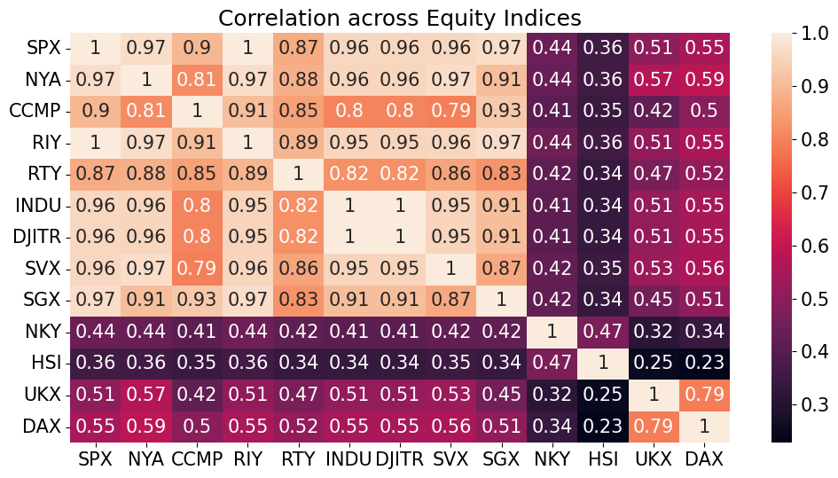
sns.heatmap(rets_index.corr(),annot=True);
plt.title('Correlation across Equity Indices');
Exchange-Traded Funds#
Investors Pile Into ETFs at Record Pace Despite Market Turmoil
WSJ - May 25, 2025
U.S. exchange-traded funds have collected some $437 billion in new assets so far this year.
What’s Left to be ETF’d? WSJ - Sep 13, 2024 There’s an ETF for nearly everything, but good ones are rare.
ETFs Are Flush With New Money. Why Billions More Are Flowing Their Way
WSJ - Oct 1, 2025
Investors have plowed more than $900 billion into U.S. exchange-traded funds so far this year
Where the New ETF Money Is Going WSJ - Oct 1, 2025 Top net ETF inflows year-to-date
An exchange-traded-fund
Trades on a stock exchange
Shares of the fund which may hold a variety of assets
Can be traded intra-day
Questions#
What is an ETF?
How does an ETF compare to Mutual Funds?
Why trade ETF’s?
History#
ETFs Began trading in the U.S. in 1993.
Active-ETF’s approved in 2008.
Around 2,000 ETF’s trade in U.S. markets.
Variety#
ETFs include funds
passively tracking an index of equities
actively tracking an equity style or trading strategy (smart beta)
alternative assets
Most ETF’s track an index. ie. S&P 500, U.S. Treasury rate, BBB-AAA credit spread, etc.
Target wide variety of equity sectors and geographies.
Funds for a variety of asset classes: equities, oil, grains, credit instruments, etc.
Active ETF’s tracking a strategy.
Note that the fund expenses and liquidity vary considerably across ETFs.
Consider a few examples.
etf_info = pd.read_excel(INFILE,sheet_name=f'etf info').set_index('ticker')
etf_info[['fund_expense_ratio','eqy_dvd_yld_ind']] /= 100
etf_info.style.format({'fund_expense_ratio':'{:.2%}','eqy_dvd_yld_ind':'{:.2%}'})
| total_number_of_holdings_in_port | fund_expense_ratio | fund_asset_class_focus | fund_objective_long | eqy_dvd_yld_ind | |
|---|---|---|---|---|---|
| ticker | |||||
| SPY | 505 | 0.09% | Equity | Large-cap | 1.13% |
| UPRO | 524 | 0.91% | Equity | Large-cap | 0.90% |
| EEM | 1204 | 0.72% | Equity | Emerging Markets | 3.07% |
| VGK | 1263 | 0.06% | Equity | European Region | 1.51% |
| EWJ | 185 | 0.50% | Equity | Japan | 2.88% |
| IYR | 67 | 0.39% | Equity | Real Estate | 1.51% |
| DBC | 28 | 0.87% | Commodity | Broad Based | 5.15% |
| HYG | 1271 | 0.49% | Fixed Income | Corporate | 5.68% |
| TIP | 52 | 0.18% | Fixed Income | Inflation Protected | 3.03% |
| BITO | 5 | 0.95% | Alternative | nan | 54.92% |
Mutual Funds vs ETFs#
ETF’s directly trade unit blocks of the assets, for authorized participants.
Allows intra-day trading.
No cash-management for redemption, load, fee, etc.
No direct redemption means favorable capital-gains treatment.
Liquidity
Reduce idiosyncratic risk.
Exchange-traded (U.S.)
Allow for wide variety of trading strategies.
Indexes vs ETFs#
Timing#
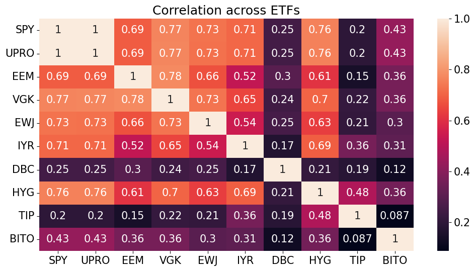
Above we saw low correlation between equity indexes in the U.S. versus Europe, partly due to asynchronous trading across time-zones.
Below, note that the correlation between SPY, VGK, and EWJ is much higher.
etfs = pd.read_excel(INFILE,sheet_name=f'etf history').set_index('date')
rets_etf = etfs.pct_change().dropna()
sns.heatmap(rets_etf.corr(),annot=True);
plt.title('Correlation across ETFs');
/var/folders/zx/3v_qt0957xzg3nqtnkv007d00000gn/T/ipykernel_40635/1376750157.py:2: FutureWarning: The default fill_method='pad' in DataFrame.pct_change is deprecated and will be removed in a future version. Either fill in any non-leading NA values prior to calling pct_change or specify 'fill_method=None' to not fill NA values.
  rets_etf = etfs.pct_change().dropna()
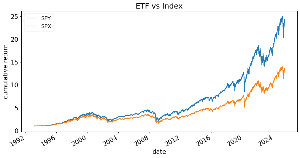
SPX vs SPY?#
If we need a benchmark for a strategy, should we use SPX or SPY?
Why do they seem to have different return statistics below?
spy_vs_spx = pd.concat([etfs[['SPY']],indexes[['SPX']]],axis=1).dropna().pct_change()
performanceMetrics(spy_vs_spx,annualization=252).style.format('{:.1%}')
| Mean | Vol | Sharpe | Min | Max | |
|---|---|---|---|---|---|
| SPY | 11.6% | 18.8% | 61.9% | -10.9% | 14.5% |
| SPX | 9.8% | 18.5% | 52.7% | -12.0% | 11.6% |
(spy_vs_spx+1).cumprod().plot(title='ETF vs Index',ylabel='cumulative return');
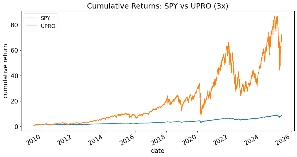
Levered ETFs#
Levered ETFs seek to provide levered exposure to an index, such as the SPX.
These include inverse-levered ETFs.
spy_vs_letf = etfs[['SPY','UPRO']].dropna()
temp = (spy_vs_letf.pct_change()+1).cumprod()
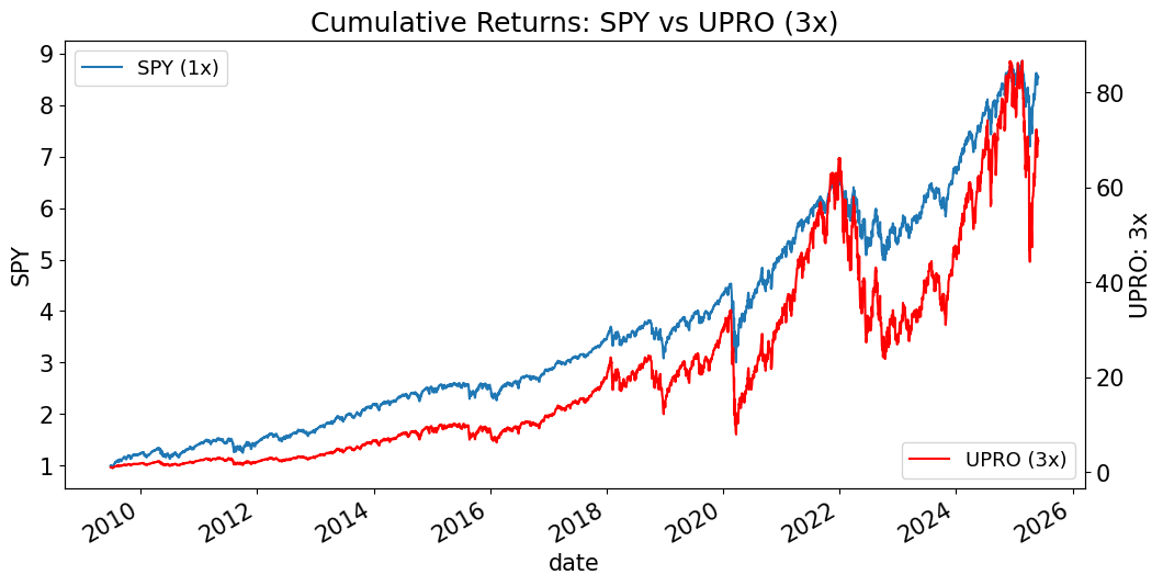
temp.plot(title='Cumulative Returns: SPY vs UPRO (3x)',ylabel='cumulative return');
fig, ax = plt.subplots()
temp[['SPY']].plot(ax=ax,ylabel='SPY');
ax.legend(['SPY (1x)'],loc='upper left')
ax2 = plt.twinx(ax=ax)
temp[['UPRO']].plot(ax=ax2,color='r',ylabel='UPRO: 3x');
ax2.legend(['UPRO (3x)'],loc='lower right');
plt.title('Cumulative Returns: SPY vs UPRO (3x)');
performanceMetrics(spy_vs_letf.pct_change(),annualization=252).style.format('{:.1%}')
| Mean | Vol | Sharpe | Min | Max | |
|---|---|---|---|---|---|
| SPY | 15.0% | 17.4% | 86.3% | -10.9% | 10.5% |
| UPRO | 40.5% | 52.1% | 77.7% | -34.9% | 28.0% |
More on LETFs#
For more on the subtleties and dangers of Levered ETFs, see the extra notebook.