Leveraged ETFs: The Compounding Problem

Billions Flowed Into New Leveraged ETFs Last Year. Now They’re in Free Fall. WSJ - March 20, 2025 Wall Street’s newest roller-coaster trade, the leveraged single-stock ETF, is plunging.

The Hidden Cost of Playing the Stock Market’s Slot Machine WSJ - Oct 3, 2025 Superpowered ETFs make money fast, but cost more than you know

How Booming Leveraged Funds Can Incinerate Your Money
WSJ - Dec 11, 2024 Variants soon might include long-short funds

How Index‑Fund Investing Turned Into an Extreme Sport
WSJ - July 11, 2025
Exchange-traded funds are becoming far more concentrated, amplifying risks.

import pandas as pd
import numpy as np
import datetime

import matplotlib.pyplot as plt
%matplotlib inline
plt.rcParams['figure.figsize'] = (8,4)
plt.rcParams['font.size'] = 12
plt.rcParams['legend.fontsize'] = 12

from cmds.portfolio import performanceMetrics, tailMetrics, maximumDrawdown, get_ols_metrics

The Math Behind the Problem

Traditional Leverage vs. Leveraged ETFs

Traditional leverage: Borrow money once, hold the position $\(r_{0,T}^{\text{Traditional}} = w \cdot [(1+r_1)(1+r_2)\cdots(1+r_T) - 1]\)$

Leveraged ETF: Rebalance the leverage daily
$\(r_{0,T}^{\text{LETF}} = (1+w \cdot r_1)(1+w \cdot r_2)\cdots(1+w \cdot r_T) - 1\)$

The Key Insight

These are NOT the same!
Daily rebalancing creates compounding effects that can work against you, especially during volatile periods.

A Simple Example

Let’s see this in action with 3x leverage over 2 days:

Traditional 3x leverage:
$\(3r_1 + 3r_2 + 3r_1r_2\)$

3x Leveraged ETF:
$\(3r_1 + 3r_2 + 9r_1r_2\)$

The difference: \(6r_1r_2\)

When returns have opposite signs (common in volatile markets), this difference hurts the LETF.

Illustration

Suppose the following…

leverage = 3
r1 = .1
r2 = -.05
cumret = (1+r1)*(1+r2) - 1
leveraged_cumret = leverage * cumret
letf_cumret = (1+leverage*r1)*(1+leverage*r2) - 1
diff = -(leverage*(leverage-1)) * r1*r2

df = pd.DataFrame([leverage, r1, r2, cumret, leveraged_cumret, letf_cumret, diff], index=['Leverage', 'r1', 'r2', 'Cumulative Return', 'Levered Cumulative Return', 'LETF Cumulative Return', 'Difference'],columns=['illustration'])
display(df.style.format('{:.1%}'))

	illustration
Leverage	300.0%
r1	10.0%
r2	-5.0%
Cumulative Return	4.5%
Levered Cumulative Return	13.5%
LETF Cumulative Return	10.5%
Difference	3.0%

What just happened?

The LETF lost 3% due to daily rebalancing! This is the volatility drag effect.

The Bottom Line

Leveraged ETFs are NOT long-term investments

• Daily rebalancing creates compounding drag
• Volatility amplifies the decay effect
• Time works against you - the longer you hold, the worse it gets
• Use case: Short-term tactical trades, not buy-and-hold

The math doesn’t lie: \((1+3r_1)(1+3r_2) \neq 1 + 3(r_1 + r_2)\) when \(r_1 \cdot r_2 \neq 0\)

Levered SPX

Let’s examine actual leveraged ETFs to see this effect in practice.

ETFs we’re analyzing:

• UPRO: 3x Long S&P 500

• SPXU: 3x Inverse S&P 500

• SPY: The underlying S&P 500 ETF

FREQ = 252

filepath_data = '../data/letf_data.xlsx'
info = pd.read_excel(filepath_data,sheet_name='descriptions')
info.set_index('ticker',inplace=True)
info.rename(columns={'trailingAnnualDividendYield':'dvd yield'},inplace=True)


rets = pd.read_excel(filepath_data,sheet_name='total returns')
rets.set_index('date',inplace=True)
rets.dropna(inplace=True)

info.loc[['SPY','UPRO','SPXU'],:].style.format({'volume':'{:.0e}','totalAssets':'{:.0e}','dvd yield':'{:.0%}'},na_rep='')

	shortName	quoteType	currency	volume	totalAssets	longBusinessSummary
ticker
SPY	SPDR S&P 500	ETF	USD	6e+07	6e+11	The trust seeks to achieve its investment objective by holding a portfolio of the common stocks that are included in the index, with the weight of each stock in the portfolio substantially corresponding to the weight of such stock in the index.
UPRO	ProShares UltraPro S&P 500	ETF	USD	4e+06	5e+09	The fund invests in financial instruments that ProShare Advisors believes, in combination, should produce daily returns consistent with the Daily Target. The index is designed to measure the performance of 500 of the largest companies listed and domiciled in the U.S. Under normal circumstances, the fund will obtain leveraged exposure to at least 80% of its total assets in components of the index or in instruments with similar economic characteristics. The fund is non-diversified.
SPXU	ProShares UltraPro Short S&P500	ETF	USD	2e+07	5e+08	The fund invests in financial instruments that ProShare Advisors believes, in combination, should produce daily returns consistent with the Daily Target. The index is designed to measure the performance of the 500 largest companies listed and domiciled in the U.S. Under normal circumstances, the fund will obtain inverse leveraged exposure to at least 80% of its total assets in components of the index or in instruments with similar economic characteristics. The fund is non-diversified.

spy = rets[['SPY','UPRO','SPXU']].copy()
spy['SPY 3x'] = 3 * spy['SPY']
spy['SPY -3x'] = -3 * spy['SPY']

spy_cumrets = ((spy+1).cumprod()-1)
spy_cumrets.plot(logy=False)
plt.show()

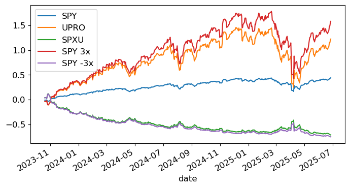
Key insight: Look at how the leveraged ETFs track against theoretical 3x performance.

cumrets = (1+spy).cumprod()
cumrets[['SPY 3x','UPRO']].plot(title='Positive Levered S&P')
plt.show()

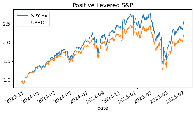
What we’re seeing: The leveraged ETFs consistently underperform their theoretical targets during volatile periods.

cumrets[['SPY -3x','SPXU']].plot(title='Inverse Levered S&P')
plt.show()

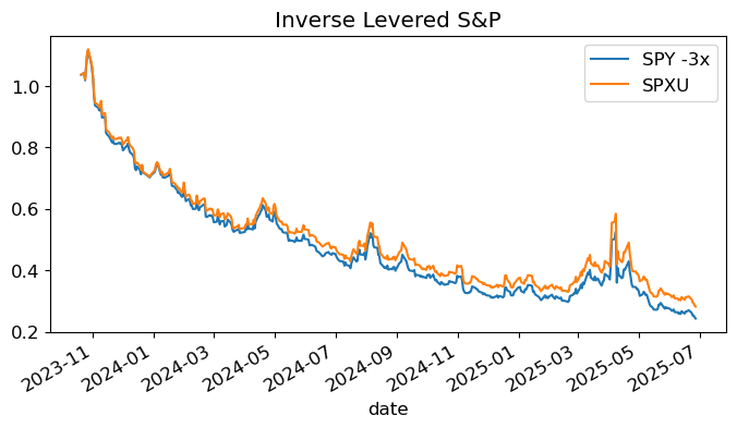
The decay effect: Over time, leveraged ETFs lose value relative to simple leveraged positions due to daily rebalancing.

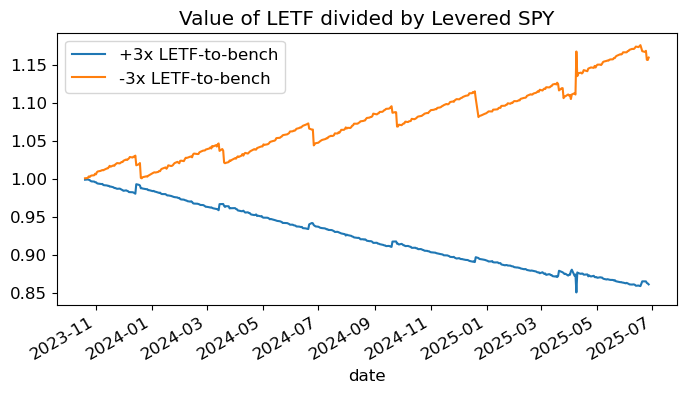
Performance Breakdown

cumrets_decay = pd.DataFrame((cumrets['UPRO'] / cumrets['SPY 3x']), columns=['+3x LETF-to-bench'])
cumrets_decay['-3x LETF-to-bench'] = (cumrets['SPXU'] / cumrets['SPY -3x'])

cumrets_decay.plot(title='Value of LETF divided by Levered SPY');

Risk-Return Analysis

performanceMetrics(spy,annualization=FREQ).style.format("{:.1%}")

	Mean	Vol	Sharpe	Min	Max
SPY	23.4%	17.3%	134.7%	-5.9%	10.5%
UPRO	60.2%	50.1%	120.3%	-17.4%	28.0%
SPXU	-62.5%	50.1%	-124.7%	-28.0%	18.2%
SPY 3x	70.1%	52.0%	134.7%	-17.6%	31.5%
SPY -3x	-70.1%	52.0%	-134.7%	-31.5%	17.6%

maximumDrawdown(spy).style.format({'Max Drawdown': "{:.1%}","Peak": "{:%Y-%m-%d}",'Bottom': "{:%Y-%m-%d}",'Recover':"{:%Y-%m-%d}"},na_rep='')

	Max Drawdown	Peak	Bottom	Recover	Duration (to Recover)
SPY	-19.0%	2025-02-19	2025-04-08	2025-06-27	128 days 00:00:00
UPRO	-49.1%	2024-12-06	2025-04-08
SPXU	-74.8%	2023-10-27	2025-06-27
SPY 3x	-48.7%	2025-02-19	2025-04-08
SPY -3x	-78.2%	2023-10-27	2025-06-27

get_ols_metrics(spy['SPY'],spy,annualization=12).drop(columns=['Treynor Ratio','Info Ratio']).style.format('{:.1%}')

	alpha	SPY	r-squared
SPY	-0.0%	100.0%	100.0%
UPRO	-0.3%	288.0%	99.5%
SPXU	0.2%	-287.4%	98.9%
SPY 3x	-0.0%	300.0%	100.0%
SPY -3x	0.0%	-300.0%	100.0%

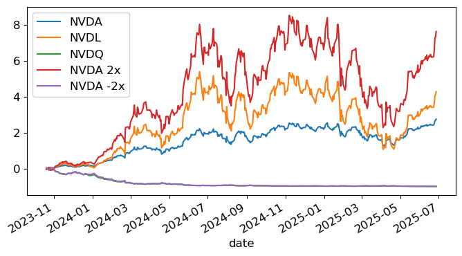
LETF for Single-Name Stock

rets['NVDA 2x'] = 2 * rets['NVDA']
rets['NVDA -2x'] = -2 * rets['NVDA']

rets['SPY 2x'] = 2 * rets['SPY']
rets['SPY -2x'] = -2 * rets['SPY']

nvda = rets[['NVDA','NVDL','NVDQ','NVDA 2x','NVDA -2x']]
nvda_cumrets = ((nvda+1).cumprod()-1)
nvda_cumrets.plot(logy=False)
plt.show()

nvda_cumrets_decay = pd.DataFrame((nvda_cumrets['NVDL'] / nvda_cumrets['NVDA 2x']), columns=['+2x'])
nvda_cumrets_decay['-2x'] = (nvda_cumrets['NVDQ'] / nvda_cumrets['NVDA -2x'])

nvda_cumrets_decay.plot(title='Value of LETF divided by Levered SPY');

get_ols_metrics(nvda['NVDA'],nvda,annualization=FREQ).drop(columns=['Treynor Ratio','Info Ratio']).style.format('{:.1%}')

	alpha	NVDA	r-squared
NVDA	-0.0%	100.0%	100.0%
NVDL	-27.4%	195.9%	99.0%
NVDQ	-2.7%	-199.6%	99.2%
NVDA 2x	-0.0%	200.0%	100.0%
NVDA -2x	0.0%	-200.0%	100.0%

SEC Statement on Single-Stock Levered and/or Inverse ETFs SEC - July 8, 2022

SEC Updated Investor Bulletin: Leveraged and Inverse ETFs
SEC - Aug 29, 2023