Currency and FX#
import pandas as pd
import numpy as np

import matplotlib.pyplot as plt
%matplotlib inline
plt.rcParams['figure.figsize'] = (10,5)
plt.rcParams['font.size'] = 13
plt.rcParams['legend.fontsize'] = 13

from cmds.portfolio import performanceMetrics, tailMetrics
Currency#
Currency is traded on the spot market at the exchange rate.
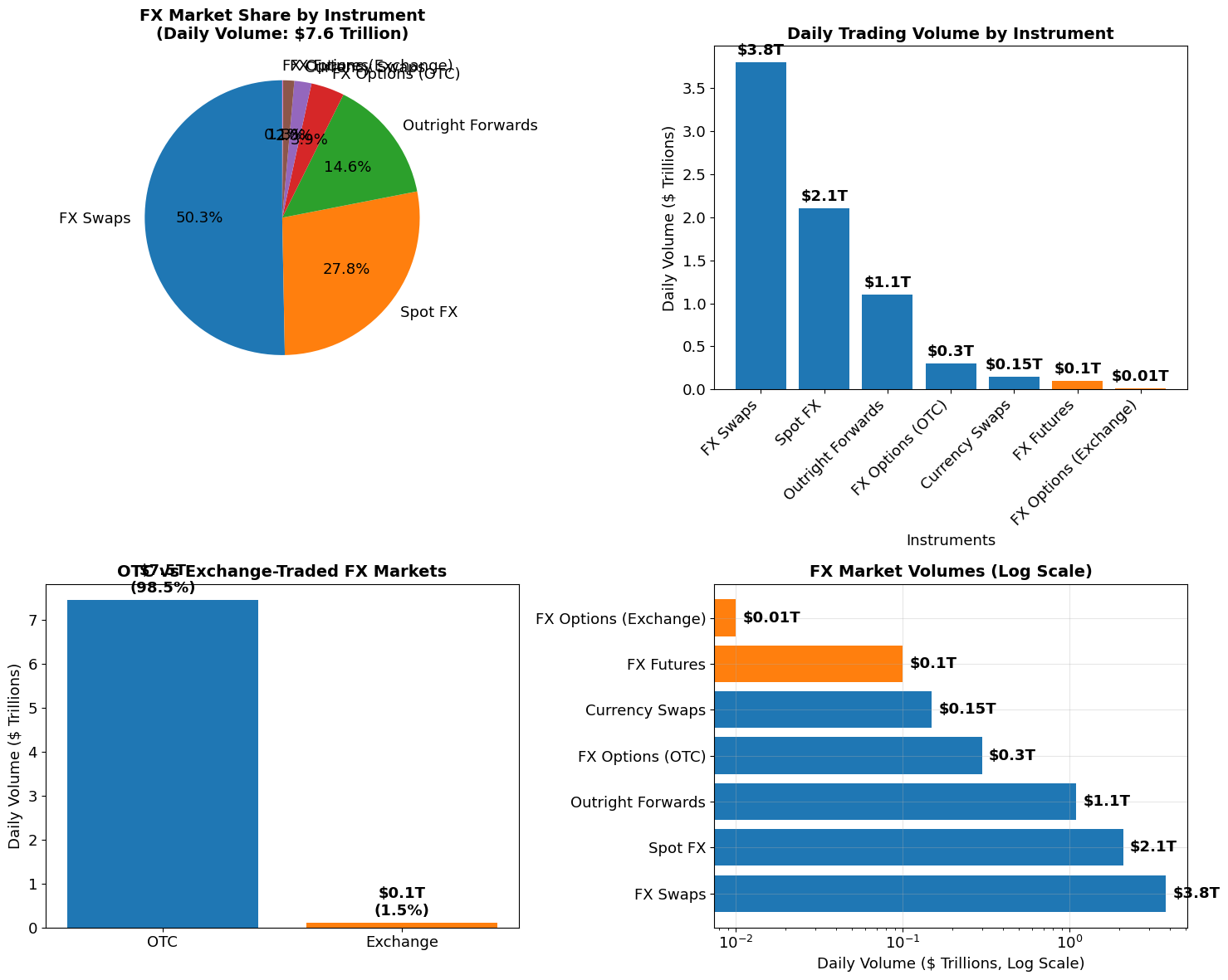
Market Size by Instrument (2022 Data)#
Total Daily FX Turnover: $7.6 trillion/day
Instrument |
Daily Volume |
% of Total |
Market Type |
Source URL |
|---|---|---|---|---|
FX Swaps |
$3.8 trillion |
50.0% |
OTC |
|
Spot FX |
$2.1 trillion |
27.6% |
OTC |
|
Outright Forwards |
$1.1 trillion |
14.5% |
OTC |
|
FX Options (OTC) |
$0.3 trillion |
3.9% |
OTC |
|
Currency Swaps |
$0.15 trillion |
2.0% |
OTC |
|
FX Futures |
~$0.1 trillion |
~1.3% |
Exchange |
|
FX Options (Exchange) |
<$0.01 trillion |
<0.1% |
Exchange |
Exchange-Traded FX Derivatives Note:#
Total exchange-traded FX volume (2021): 5.54 billion contracts - includes both futures and options, but heavily weighted toward futures. Exchange-traded FX options volume is minimal compared to OTC (\(300B/day vs <\)10B/day estimated).
Key Market Features#
OTC completely dominates: 98.6%+ of FX trading is over-the-counter
FX Swaps largest: Short-term funding swaps are half the market
Exchange-traded tiny but growing: Futures +24% in 2022, but still <2% of total
Options mostly OTC: Exchange-traded FX options <0.1% of total market
Geographic concentration: 78% of trading in 5 centers (UK 38%, US 19%, Singapore 9%, Hong Kong 7%, Japan 4%)
# FX Market Size Visualization
import pandas as pd
import matplotlib.pyplot as plt
import numpy as np
import seaborn as sns

# Market size data (daily volumes in trillion USD)
fx_data = {
    'Instrument': ['FX Swaps', 'Spot FX', 'Outright Forwards', 'FX Options (OTC)',
                   'Currency Swaps', 'FX Futures', 'FX Options (Exchange)'],
    'Volume_Trillions': [3.8, 2.1, 1.1, 0.3, 0.15, 0.1, 0.01],
    'Market_Type': ['OTC', 'OTC', 'OTC', 'OTC', 'OTC', 'Exchange', 'Exchange'],
    'Percentage': [50.0, 27.6, 14.5, 3.9, 2.0, 1.3, 0.1]
}

fx_df = pd.DataFrame(fx_data)

# Create subplots
fig, ((ax1, ax2), (ax3, ax4)) = plt.subplots(2, 2, figsize=(15, 12))

# 1. Pie Chart - Overall Market Share
colors = ['#1f77b4', '#ff7f0e', '#2ca02c', '#d62728', '#9467bd', '#8c564b', '#e377c2']
wedges, texts, autotexts = ax1.pie(fx_df['Percentage'], labels=fx_df['Instrument'],
                                   autopct='%1.1f%%', colors=colors, startangle=90)
ax1.set_title('FX Market Share by Instrument\n(Daily Volume: $7.6 Trillion)', fontsize=14, fontweight='bold')

# 2. Bar Chart - Volume by Instrument
bars = ax2.bar(range(len(fx_df)), fx_df['Volume_Trillions'],
               color=['#1f77b4' if x == 'OTC' else '#ff7f0e' for x in fx_df['Market_Type']])
ax2.set_title('Daily Trading Volume by Instrument', fontsize=14, fontweight='bold')
ax2.set_xlabel('Instruments')
ax2.set_ylabel('Daily Volume ($ Trillions)')
ax2.set_xticks(range(len(fx_df)))
ax2.set_xticklabels(fx_df['Instrument'], rotation=45, ha='right')

# Add value labels on bars
for i, v in enumerate(fx_df['Volume_Trillions']):
    ax2.text(i, v + 0.05, f'${v}T', ha='center', va='bottom', fontweight='bold')

# 3. OTC vs Exchange Comparison
otc_total = fx_df[fx_df['Market_Type'] == 'OTC']['Volume_Trillions'].sum()
exchange_total = fx_df[fx_df['Market_Type'] == 'Exchange']['Volume_Trillions'].sum()

market_comparison = pd.DataFrame({
    'Market Type': ['OTC', 'Exchange'],
    'Volume': [otc_total, exchange_total],
    'Percentage': [otc_total/(otc_total+exchange_total)*100, exchange_total/(otc_total+exchange_total)*100]
})

bars3 = ax3.bar(market_comparison['Market Type'], market_comparison['Volume'],
                color=['#1f77b4', '#ff7f0e'])
ax3.set_title('OTC vs Exchange-Traded FX Markets', fontsize=14, fontweight='bold')
ax3.set_ylabel('Daily Volume ($ Trillions)')
for i, v in enumerate(market_comparison['Volume']):
    ax3.text(i, v + 0.1, f'${v:.1f}T\n({market_comparison["Percentage"].iloc[i]:.1f}%)',
             ha='center', va='bottom', fontweight='bold')

# 4. Log Scale View (to show smaller instruments better)
ax4.barh(fx_df['Instrument'], fx_df['Volume_Trillions'],
         color=['#1f77b4' if x == 'OTC' else '#ff7f0e' for x in fx_df['Market_Type']])
ax4.set_xscale('log')
ax4.set_title('FX Market Volumes (Log Scale)', fontsize=14, fontweight='bold')
ax4.set_xlabel('Daily Volume ($ Trillions, Log Scale)')
ax4.grid(True, alpha=0.3)

# Add value labels
for i, v in enumerate(fx_df['Volume_Trillions']):
    ax4.text(v * 1.1, i, f'${v}T', va='center', fontweight='bold')

plt.tight_layout()
plt.show()
Exchange-Traded FX Options Analysis:#
1. Total Exchange-Traded FX Volume (All Instruments):
2021 Global Total: 5.54 billion contracts (FIA Survey)
Heavily skewed toward futures (not options)
2. Exchange-Traded Options are Tiny:
Estimated daily volume: <\(10 billion (vs \)300B OTC options)
Market share: <0.1% of total FX market
Why so small?
Standardization constraints
Limited currency pairs available
Institutional preference for OTC customization
Higher liquidity in OTC markets
3. Key Exchanges for FX Options:
CME Group (dominant in FX futures, minimal options)
ICE Futures
Eurex (some currency options)
Conclusion:#
Exchange-traded FX options exist but are economically insignificant. The OTC market dominates because:
Customization: Tailored strikes, expiries, currencies
Size: Institutional-size transactions
Liquidity: 24/7 global OTC market vs exchange hours
Cost: Lower transaction costs for large trades
The $300 billion/day in OTC FX options captures >99.9% of the options market.
Data#
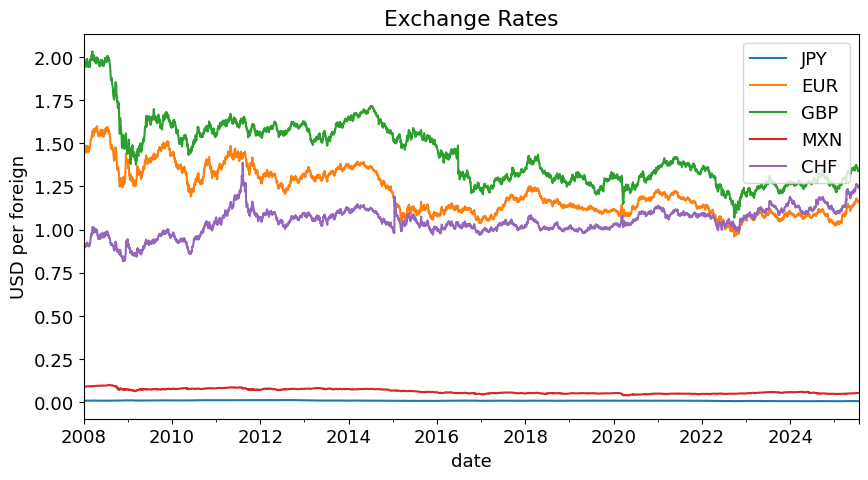
Exchange rates#
Spot exchange rates.
DATAPATH_FX = '../data/fx_data_index.xlsx'
SHEET = 'exchange rates'
fxraw = pd.read_excel(DATAPATH_FX, sheet_name=SHEET).set_index('date')
fxraw.plot(title='Exchange Rates',ylabel='USD per foreign',figsize=(10,5));
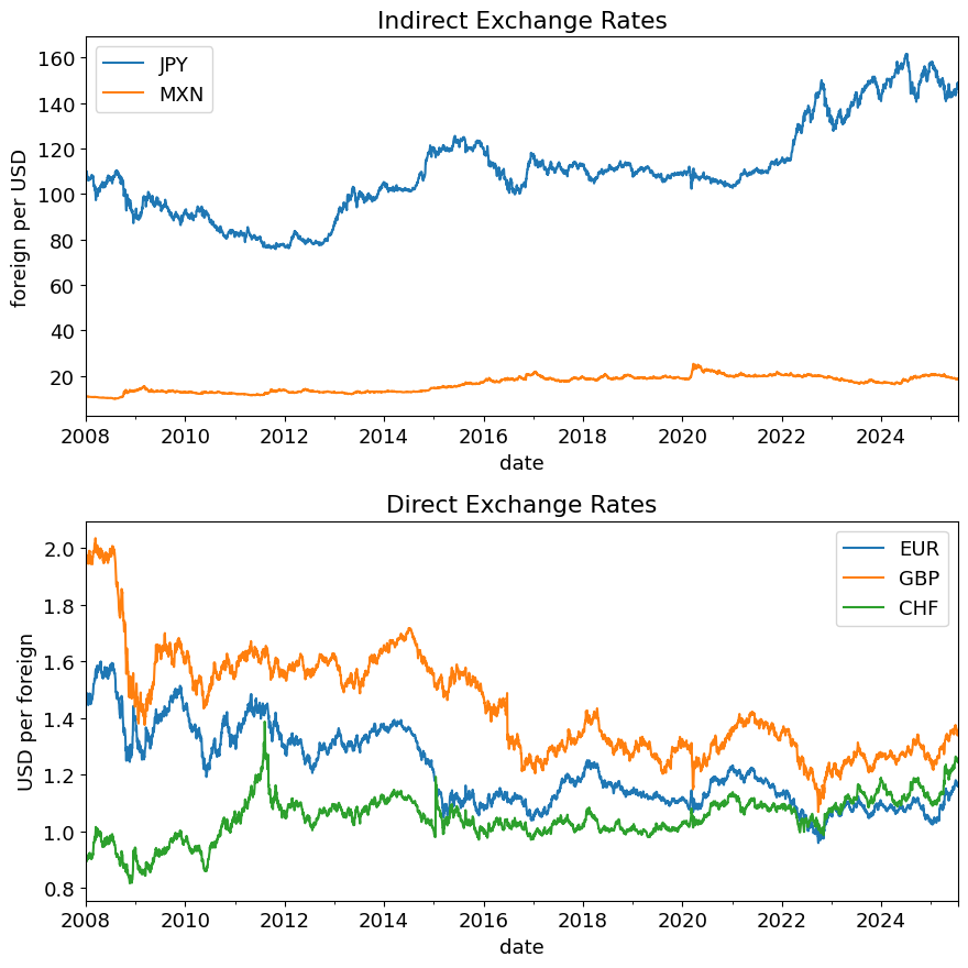
Direct vs Indirect#
idx_direct = fxraw.mean(axis=0) < .1
idx_indirect = fxraw.mean(axis=0) > .1

fig, (ax1, ax2) = plt.subplots(2,1, figsize=(9,9), sharey=False)

(1/fxraw.loc[:, idx_direct]).plot(ax=ax1, title='Indirect Exchange Rates', ylabel='foreign per USD')
fxraw.loc[:, idx_indirect].plot(ax=ax2, title='Direct Exchange Rates', ylabel='USD per foreign')

plt.tight_layout()
plt.show()
Quote Conventions#
Instrument |
Quote Convention |
|---|---|
Spot FX |
Mix (whichever historically was above 1) |
FX Forwards |
Mix (follows spot conventions for each pair) |
FX Futures |
American terms (USD per unit of foreign) |
FX Options |
American terms (USD per unit of foreign) |
Goldman’s Warrant Formula Error: A Cautionary Tale#
In February 2011, Goldman Sachs launched Nikkei warrants in Hong Kong with a critical typo in the settlement formula. Instead of dividing by the JPY/HKD exchange rate, the documentation said to multiply by it.
This error was caught and corrected two months later, but it illustrates how a simple mistake can have massive financial consequences.
The Error: Indirect vs Direct#
Correct Formula:
Settlement = (Strike - Closing) × Amount ÷ Exchange Rate
Erroneous Formula (as published):
Settlement = (Strike - Closing) × Amount × Exchange Rate
Impact:#
Let’s see what happened with Goldman’s (ID #10075) Put Warrants expiring September 9, 2011:
Market Data |
Value |
|---|---|
Strike Level |
10,000 points |
Nikkei Closing |
8,737.66 points |
Intrinsic Value |
1,262.34 points |
Currency Amount |
350 JPY per point |
Exchange Rate |
9.9264 JPY/HKD |
GSHK = pd.DataFrame([1000,10000,1/350,10000,8737.66,9.9264,7.85],index=['total lots','lot size','multiplier per lot','index strike','index close','JPY/HKD','HKD per USD'],columns=['Feb 2011'])
GSHK.style.format('{:,.2f}')
| Feb 2011 | |
|---|---|
| total lots | 1,000.00 |
| lot size | 10,000.00 |
| multiplier per lot | 0.00 |
| index strike | 10,000.00 |
| index close | 8,737.66 |
| JPY/HKD | 9.93 |
| HKD per USD | 7.85 |
value = pd.DataFrame(
    [
        GSHK.loc['index strike', 'Feb 2011'] - GSHK.loc['index close', 'Feb 2011']
    ],
    index=['intrinsic value'],
    columns=['correct']
)
value.loc['intrinsic value', 'incorrect'] = value.loc['intrinsic value', 'correct']

value.loc['yen per warrant', 'correct']   = value.loc['intrinsic value', 'correct'] * GSHK.loc['multiplier per lot', 'Feb 2011']
value.loc['yen per warrant', 'incorrect'] = value.loc['intrinsic value', 'correct'] * GSHK.loc['multiplier per lot', 'Feb 2011']

value.loc['FX rate JPY per HKD', 'correct']   = GSHK.loc['JPY/HKD', 'Feb 2011']
value.loc['FX rate JPY per HKD', 'incorrect'] = 1 / GSHK.loc['JPY/HKD', 'Feb 2011']

value.loc['HKD per warrant', 'correct']   = value.loc['yen per warrant', 'correct'] / value.loc['FX rate JPY per HKD', 'correct']
value.loc['HKD per warrant', 'incorrect'] = value.loc['yen per warrant', 'incorrect'] / value.loc['FX rate JPY per HKD', 'incorrect']

value.loc['HKD per lot', 'correct']       = value.loc['HKD per warrant', 'correct'] * GSHK.loc['lot size', 'Feb 2011']
value.loc['HKD per lot', 'incorrect']     = value.loc['HKD per warrant', 'incorrect'] * GSHK.loc['lot size', 'Feb 2011']

value.loc['HKD total issue', 'correct']   = value.loc['HKD per lot', 'correct'] * GSHK.loc['total lots', 'Feb 2011']
value.loc['HKD total issue', 'incorrect'] = value.loc['HKD per lot', 'incorrect'] * GSHK.loc['total lots', 'Feb 2011']

value.loc['USD exposure', 'correct']   = value.loc['HKD total issue', 'correct'] / GSHK.loc['HKD per USD', 'Feb 2011']
value.loc['USD exposure', 'incorrect'] = value.loc['HKD total issue', 'incorrect'] / GSHK.loc['HKD per USD', 'Feb 2011']

# Format for display
display(value.style.format('{:,.2f}'))
| correct | incorrect | |
|---|---|---|
| intrinsic value | 1,262.34 | 1,262.34 |
| yen per warrant | 3.61 | 3.61 |
| FX rate JPY per HKD | 9.93 | 0.10 |
| HKD per warrant | 0.36 | 35.80 |
| HKD per lot | 3,633.43 | 358,014.05 |
| HKD total issue | 3,633,427.74 | 358,014,050.74 |
| USD exposure | 462,857.04 | 45,606,885.44 |
Sources#
Term Sheet
https://www.hkexnews.hk/listedco/listconews/sehk/2011/0211/ltn20110211616_c.pdf
HKEX Amendment Notice LTN20110331323, March 31, 2011*
https://www.hkexnews.hk/listedco/listconews/sehk/2011/0331/ltn20110331323.pdf https://www.hkexnews.hk/listedco/listconews/sehk/2011/0331/ltn20110331323.pdf
News articles
https://www.ft.com/content/cd3551ea-3600-3d92-8382-a44b6d13dbf4
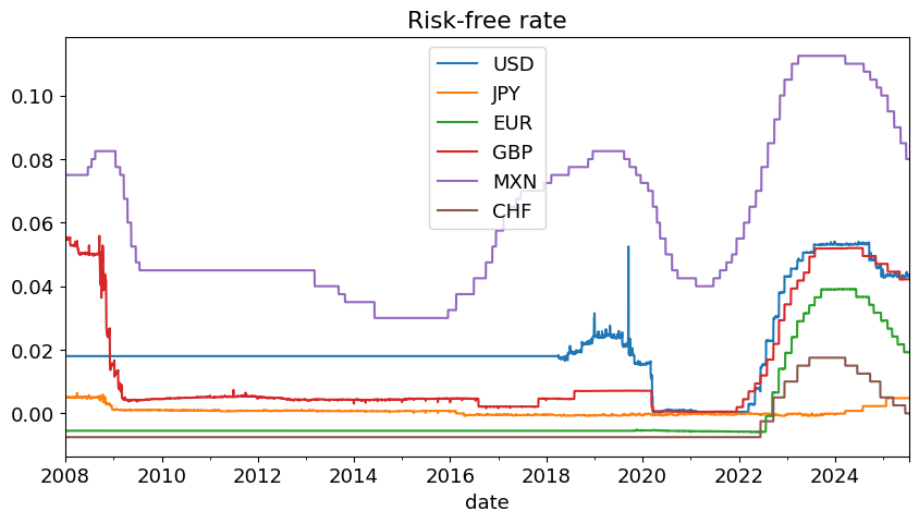
Risk-free rates#
The data reports the risk-free rates for various currencies.
Data Source: Overnight Deposit vs Index#
With LIBOR, there was a set of risk-free rates under a single, consistent methodology.
Now, we are left to get a rate from each specific currency.
Where possible, we are choosing the Bloomberg overnight deposit rate.
For some currencies, that data seems suspect, and we use an index.
SHEET = 'sources'
sources = pd.read_excel(DATAPATH_FX,sheet_name=SHEET).set_index('ticker')
display(sources.style.format(na_rep='').set_caption('Sources for Risk-free Rates'))
| selected | name | long name | sec des | index source | country | currency | quote currency | |
|---|---|---|---|---|---|---|---|---|
| ticker | ||||||||
| ESTRON Index | yes | ESTR Volume Weighted Trimmed M | ESTR Volume Weighted Trimmed Mean Rate | ESTR Volume Weighted Trimmed M | European Central Bank | TE | EUR | |
| MUTKCALM Index | yes | Bank of Japan Final Result: Un | Bank of Japan Final Result: Unsecured Overnight Call Rate TONAR | Bank of Japan Final Result: Un | Bank of Japan | JN | JPY | |
| MXONBR Index | yes | Bank of Mexico Official Overni | Bank of Mexico Official Overnight Rate | Bank of Mexico Official Overni | Banco de Mexico | MX | MXN | |
| SOFRRATE Index | yes | United States SOFR Secured Ove | United States SOFR Secured Overnight Financing Rate | United States SOFR Secured Ove | Federal Reserve Bank of New Yo | US | USD | |
| SONIO/N Index | yes | SONIA Interest Rate Benchmark | SONIA Interest Rate Benchmark | SONIA Interest Rate Benchmark | Bank of England | GB | GBP | |
| SZLTDEP Index | yes | Swiss National Bank Policy Rat | Swiss National Bank Policy Rate Decision | Swiss National Bank Policy Rat | Swiss National Bank | SZ | CHF | |
| BPDR1T CMPN Curncy | no | GBP DEPOSIT O/N | GBP Overnight Deposit | BPDR1T Curncy | GB | GBP | USD | |
| EUDR1T CMPN Curncy | no | EUR DEPOSIT O/N | EUR Overnight Deposit | EUDR1T Curncy | EU | EUR | USD | |
| JYDR1T CMPN Curncy | no | JPY DEPOSIT O/N | JPY Overnight Deposit | JYDR1T Curncy | JP | JPY | USD | |
| MPDR1T CMPN Curncy | no | MXN Deposit ON | MXN Overnight Deposit | MPDR1T Curncy | MX | MXN | USD | |
| SFDR1T CMPN Curncy | no | CHF DEPOSIT O/N | CHF Overnight Deposit | SFDR1T Curncy | CH | CHF | USD | |
| USDR1T CMPN Curncy | no | USD DEPOSIT O/N | USD Overnight Deposit | USDR1T Curncy | US | USD | USD |
Data Note: Timing#
The data is defined such that the March value of the risk-free rate corresponds to the rate beginning in March and ending in April.
In terms of the class notation, \(r^{f,i}_{t,t+1}\) is reported at time \(t\). (It is risk-free, so it is a rate from \(t\) to \(t+1\) but it is know at \(t\).
SHEET = 'risk-free rates'
rfraw = pd.read_excel(DATAPATH_FX,sheet_name=SHEET).set_index('date')
rfraw.tail().style.format('{:.2%}').format_index(lambda x: x.strftime('%Y-%m-%d'))
| USD | JPY | EUR | GBP | MXN | CHF | |
|---|---|---|---|---|---|---|
| date | ||||||
| 2025-07-14 | 4.33% | 0.48% | 1.92% | 4.22% | 8.00% | 0.00% |
| 2025-07-15 | 4.37% | 0.48% | 1.92% | 4.22% | 8.00% | 0.00% |
| 2025-07-16 | 4.34% | 0.48% | 1.92% | 4.22% | 8.00% | 0.00% |
| 2025-07-17 | 4.34% | 0.48% | 1.93% | 4.22% | 8.00% | 0.00% |
| 2025-07-18 | 4.30% | 0.48% | 1.92% | 4.22% | 8.00% | 0.00% |
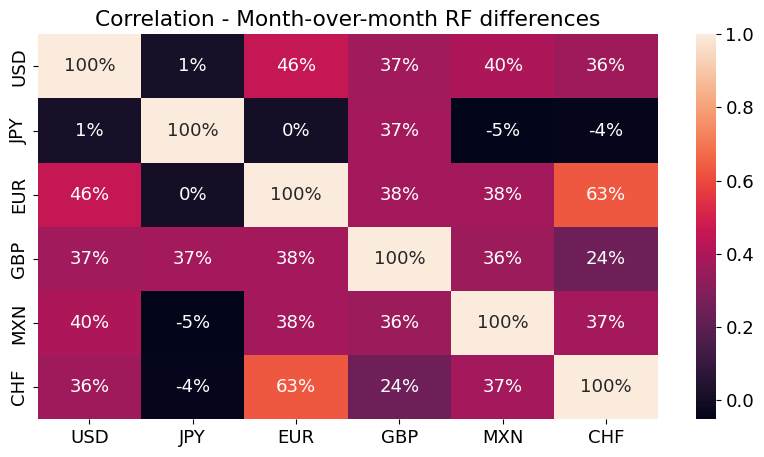
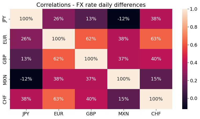
Visualizing the Data#
rfraw.plot(title='Risk-free rate',figsize=(10,5));
sns.heatmap(rfraw.diff().corr(),annot=True,fmt='.0%')
plt.title('Correlations - Day-over-day RF Differences')
plt.show()

temp = rfraw.resample('ME').last()
sns.heatmap(temp.diff().corr(),annot=True,fmt='.0%')
plt.title('Correlation - Month-over-month RF differences')
plt.show()
sns.heatmap(fxraw.diff().corr(),annot=True,fmt='.0%')
plt.title('Correlations - FX rate daily differences');
Returns on Holding Currency#
Notation#
\(S_t\) denotes the foreign exchange rate, expressed as USD per foreign currency
\(\RF_{t,t+1}\) denotes the risk-free factor on US dollars (USD).
\(\RFa_{t,t+1}\) denotes the risk-free factor on a particular foreign currency.
Two components to returns#
Misconception that the return on currency is the percentage change in the exchange rate:
The price of the currency is \(S_t\) dollars.
In terms of USD, the payoff at time t + 1 of the Euro riskless asset is
That is,
we capitalize any FX gains,
but we also earn the riskless return accumulated by the foreign currency.
Thus, the USD return on holding Euros is given by,
shared_indexes = rfraw.index.intersection(fxraw.index)

# Split the merged DataFrame back into the original two DataFrames with shared indexes
rf = rfraw.loc[shared_indexes,:]
fx = fxraw.loc[shared_indexes,:]
USDRF = 'USD'

DAYS = fx.resample('YE').size().median()
rf /= DAYS

rfusd = rf[[USDRF]]
rf = rf.drop(columns=[USDRF])

fxgrowth = (fx / fx.shift())
rets = fxgrowth.mul(1+rf.values,axis=1) - 1
rx = rets.sub(rfusd.values,axis=1)
fig, ax = plt.subplots()
(1+rets).cumprod().plot(ax=ax)
(1+rfusd).cumprod().plot(ax=ax)
plt.title('Cumulative Returns of FX')
plt.ylabel('cumulative return')
plt.figsize=(10,5)
plt.show()
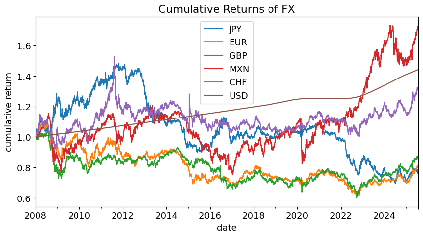
Extra Statistics on Returns#
Main takeaway:
small mean return–only exciting if you use leverage
substantial volatility
large drawdowns (tail-events)
tabmets = performanceMetrics(rx,annualization=DAYS)[['Mean','Vol','Min','Max']]
pd.concat([tabmets,tailMetrics(rets)['Max Drawdown']],axis=1).style.format('{:.1%}').set_caption('Daily Excess Returns - Currency')
| Mean | Vol | Min | Max | Max Drawdown | |
|---|---|---|---|---|---|
| JPY | -3.2% | 10.1% | -5.3% | 3.9% | -53.1% |
| EUR | -2.9% | 9.2% | -2.4% | 3.5% | -44.5% |
| GBP | -2.5% | 9.6% | -8.1% | 3.1% | -42.3% |
| MXN | 1.9% | 13.1% | -7.6% | 6.9% | -37.8% |
| CHF | 0.0% | 11.0% | -8.7% | 21.5% | -34.4% |
Decomposing the Returns#
Using logs, we can split out the two components of excess log returns
Logarithms#
The data is mostly analyzed in logs, as this simplifies equations later.
For monthly rates, logs vs levels won’t make a big difference.
Excess returns#
The (USD) return in excess of the (USD) risk-free rate is then
Two spreads#
For convenience, rewrite this as
Data Consideration#
Build the spread in risk-free rates:
Lag this variable, so that the March-to-April value is stamped as April.
Build the FX growth rates:
These are already stamped as April for the March-to-April FX growth.
Then the excess log return is simply the difference of the two objects.
logFX = np.log(fx)
logRFraw = np.log(rfraw+1)
logRFusd = logRFraw[[USDRF]]
logRF = logRFraw.drop(columns=[USDRF])
logRFusd = np.log(rfusd+1)
logRF = np.log(rf+1)
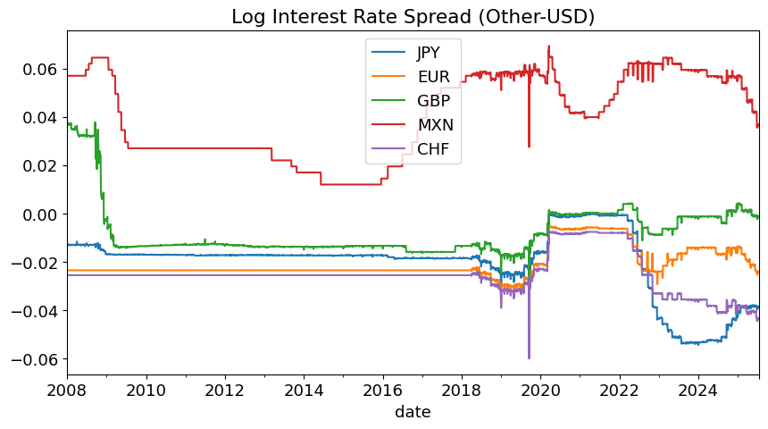
logRFspread = -logRF.subtract(logRFusd.values,axis=0)
logRFspread = logRFspread.shift(1)
logFXgrowth = logFX.diff(axis=0)
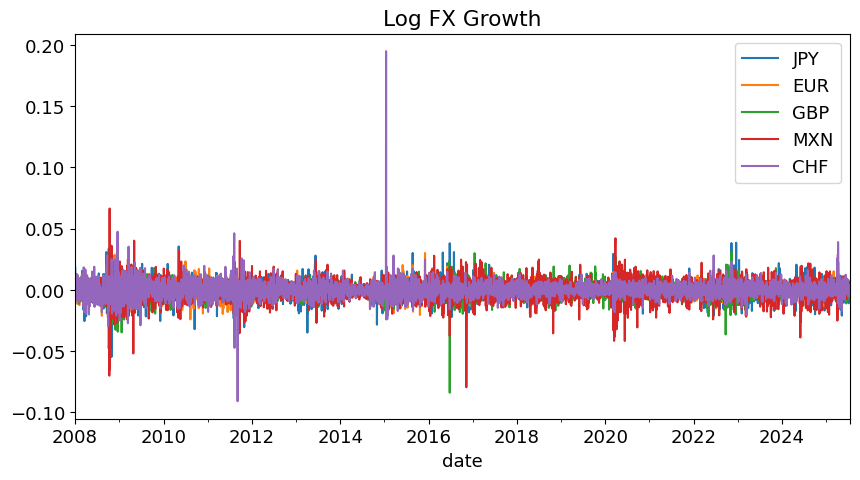
logRX = logFXgrowth - logRFspread.values
logFXgrowth.plot(title='Log FX Growth', figsize=(10,5))
plt.show()
(-logRFspread*DAYS).plot(title='Log Interest Rate Spread (Other-USD)', figsize=(10,5));
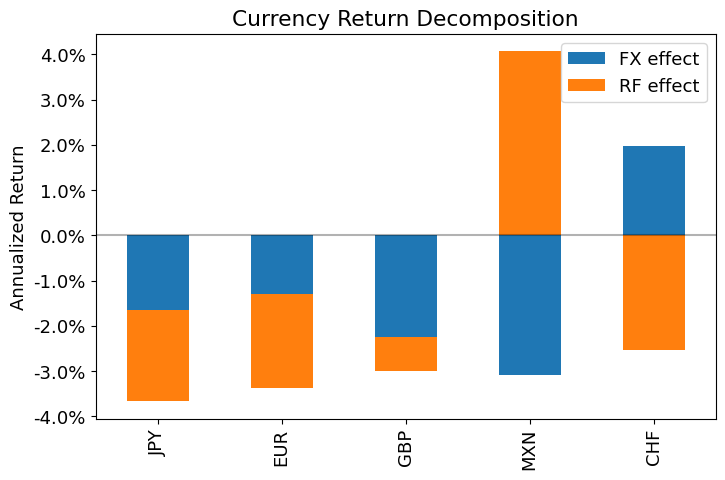
rx_components = logFXgrowth.mean().to_frame()
rx_components.columns=['FX effect']
rx_components['RF effect'] = -logRFspread.mean().values
rx_components['Total'] = rx_components.sum(axis=1)
rx_components *= DAYS

ax = rx_components[['FX effect', 'RF effect']].plot(kind='bar', stacked=True, figsize=(8, 5))
plt.title('Currency Return Decomposition')
plt.ylabel('Annualized Return')
plt.axhline(0, color='black', alpha=0.3)
ax.yaxis.set_major_formatter(plt.FuncFormatter(lambda y, _: '{:.1%}'.format(y)))
plt.show()

display(rx_components.style.format('{:.2%}'))
| FX effect | RF effect | Total | |
|---|---|---|---|
| JPY | -1.64% | -2.03% | -3.67% |
| EUR | -1.30% | -2.07% | -3.36% |
| GBP | -2.24% | -0.75% | -2.99% |
| MXN | -3.08% | 4.07% | 0.99% |
| CHF | 1.98% | -2.53% | -0.56% |
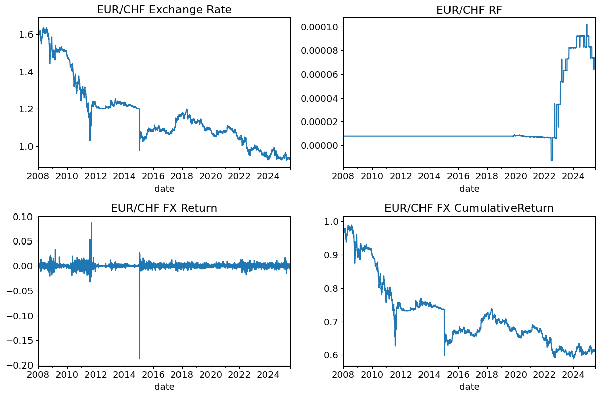
Carry Trade: EUR-CHF#
Consider a trade…
long
EURshort
CHF
EUR_CHF = (fx['EUR'] / fx['CHF'])
EUR_CHF_RF = (rf['EUR'] - rf['CHF'])
EUR_CHF_RETS = (1+EUR_CHF.pct_change()) * (1+rf['EUR']) - (1+rf['CHF'])

fig, ((ax1, ax2), (ax3, ax4)) = plt.subplots(2, 2, figsize=(12, 8))

# Plot each series on its respective subplot
EUR_CHF.plot(ax=ax1, title='EUR/CHF Exchange Rate')
EUR_CHF_RF.plot(ax=ax2, title='EUR/CHF RF')
EUR_CHF_RETS.plot(ax=ax3, title='EUR/CHF FX Return')
(1+EUR_CHF_RETS).cumprod().plot(ax=ax4, title='EUR/CHF FX Cumulative Return')

plt.tight_layout()
plt.show()
Covered Interest Parity#
Currency Forwards#
Let \(\Fcrncy_t\) denote the forward rate on the one-period FX contract, \(S_{t+1}\).
The forward FX rate, \(\Fcrncy\), is a rate contracted at time t regarding the exchange of currency at some future time, t + k .
Here, we just consider one-period forward rates. That is, where \(T_2\) is \(T_1+1\).
The superscript $ is simply to distinguish this as an FX forward versus an interest rate forward.
Pricing Equation#
Covered Interest Parity is a market relationship between exchange rates and risk-free rates.
In logs,
or rather, the forward-premium equals the interest rate differential:
CIP and No Arbitrage#
Consider two ways of moving USD from t to t + 1.
Invest in the USD risk-free rate.
Invest in the Euro risk-free rate.
Buy Euros, invest in the Euro risk-free rate
simultaneously use a forward contract to lock in the time t + 1 price of selling the Euros back for USD.
The second strategy replicates the first, so CIP follows just from no arbitrage, (Law of One Price.)
Takeaway#
Due to Covered Interest Parity,
Pricing the forward on FX is easy: just look at the current exchange rate and the interest rate differential.
The forward premium (spread between forward and spot) is often used to measure the difference in interest rates across countries.
Cryptocurrency#
Crypto Data#
For a more thorough description of Crypto, see the references below.
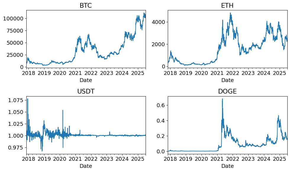
Here, we simply look at the data of the 4 largest cryptocurrencies.
LOADFILE = '../data/crypto_data.xlsx'
crypto = pd.read_excel(LOADFILE,sheet_name='prices').set_index('Date')
crypto.index = pd.to_datetime(crypto.index)
crypto.columns = crypto.columns.str.split('-').str[0]
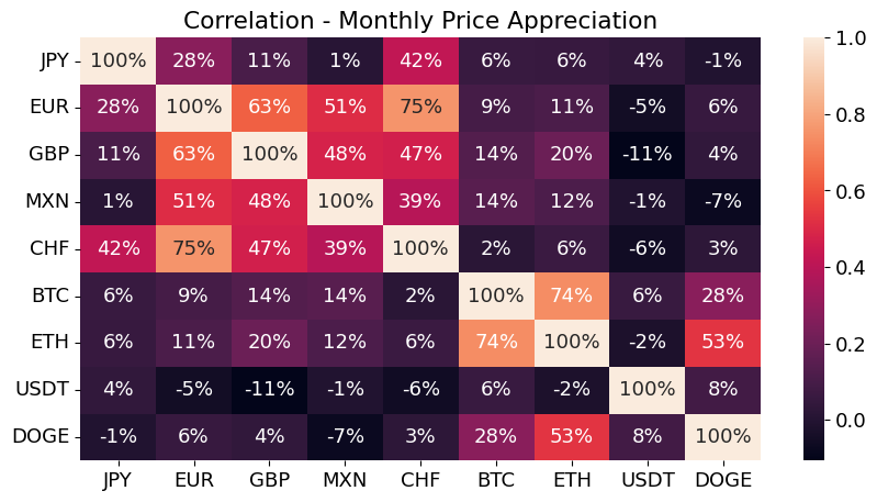
currency = pd.concat([fx,crypto],axis=1)

sns.heatmap(currency.resample('ME').last().pct_change(fill_method=None).corr(),annot=True,fmt='.0%');
plt.title('Correlation - Monthly Price Appreciation');
fig, ax = plt.subplots(2,2,figsize=(10,6))
for i, col in enumerate(crypto.columns):
    crypto[col].plot(ax=ax[int(i/2),i%2], title=col)

plt.tight_layout()
plt.show()
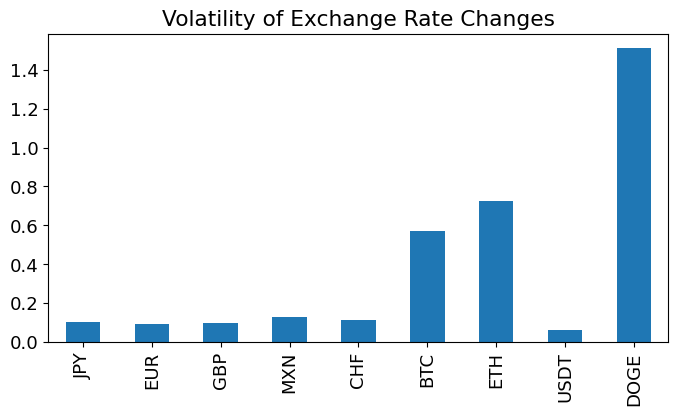
ANNUALIZE= np.sqrt(252)
(currency.pct_change(fill_method=None).std()*ANNUALIZE).plot.bar(title='Volatility of Exchange Rate Changes',figsize=(8,4))
plt.show()