Stocks#
import pandas as pd
import numpy as np
import datetime
import warnings

from sklearn.linear_model import LinearRegression
from sklearn.decomposition import PCA
from scipy.optimize import minimize

import matplotlib.pyplot as plt
%matplotlib inline
plt.rcParams['figure.figsize'] = (12,6)
plt.rcParams['font.size'] = 15
plt.rcParams['legend.fontsize'] = 13

from matplotlib.ticker import (MultipleLocator,
                               FormatStrFormatter,
                               AutoMinorLocator)

import seaborn as sns

import sys
sys.path.insert(0, '../cmds')
from utils import *
from portfolio import *
Equities#
Capital Structure#
Funding#
Assets are funded by investors, primarily via one of two types of investor claims:
debt - senior, fixed (scheduled) claim
equity - junior, residual claim
This is true of any assets, including
publicly-listed companies
privately-listed companies
private equity funds
hedge funds
Stocks#
Stocks are equity claims on assets of a corporation.
Stockholders have a junior claim on the assets and income of the firm.
Namely, they receive whatever is left over after all other claimants (suppliers, tax collectors, creditors, etc.) have been paid.
The firm can pay out the residual as dividends or reinvest it in the firm which increases the value of the shares.
Limited Liability#
Limited liability means that shareholders are not accountable for a firm’s obligations.
Losses are limited to the original investment.
Equity claim is similar to a call option on a firm’s overall value.
Compare this to unincorporated businesses where owners are personally liable.
Market size and ownership#
Of all types of capital market securities, stocks have the most market value.
However, annual new issues are much smaller than that of corporate bonds.
Annual new issues are less than 1% of the market value of equities.
About half of stocks are held by individuals.
The other half are held by institutional investors such as pension funds, mutual funds, and insurance companies.
Types of stock#
Consider two types of stock.
Common stock is a simple equity claim. It may or may not have voting rights.
Preferred stock is like a hybrid of equity and debt. Like debt, it has no voting rights.
If no specification is made, “stock” typically refers to common stock, a pure equity claim.
Preferred stock#
Consider some ways preferred is like debt and also equity.
It has a stated dividend rate, which is similar to a coupon rate on a bond.
Unlike a bond, the dividend does not have to be paid.
However, common stockholders cannot be paid dividends until preferred dividends are paid.
In fact, usually the cumulative preferred dividend must be paid first.
Tax Treatment#
Preferred stock has favorable tax treatment, which leads to special demand and supply of it.
Stock Categorization#
In trading, it is common to group equities by
geographical location
sector
size
style
A few comments on this.
Cap#
The term “cap” typically refers to equity capitalization which is the total market value of the firm’s equity.
Thus, a stock will be bucketed as small cap, mid cap, large cap.
Sector / Industry#
There are a number of common sector/industry classifications.
The Global Industry Classification Standard (GICS) is a popular classification, but there are many.
GICS has a top level of 11 Sectors subdivided by Industry Group, Industry and Sub-Industry.
Style#
Style analysis refers to grouping stocks by various measures.
Book Metrics#
“Book” measures refer to data from financial reporting (accounting).
These book measures are not the same as actual market values.
This is especially important to note for the book value of equity, the book capitalization.
Financial Statements#
balance sheet
income statment
statement of cashflows
Earnings#
For now, all that will be noted about earnings is that they are a book (accounting) measure of profits, not an actual cashflow.
Dividends are an actual market cashflow.
Book-to-Market#
The book-to-market (B/M) ratio is the market value of equity divided by the book (balance sheet) value of equity.
High B/M means strong (accounting) fundamentals per market-value-dollar.
High B/M are value stocks.
Low B/M are growth stocks.
Value and Growth#
Many other measures of value based on some cash-flow or accounting value per market price.
Earnings-price is a popular metric beyond value portfolios. Like B/M, the E/P ratio is accounting value per market valuation.
EBITDA-price is similar, but uses accounting measure of profit that ignores taxes, financing, and depreciation.
Dividend-price uses common dividends, but less useful for individual firms as many have no dividends.
Many competing claims to special/better measure of ‘value’.
Other Styles#
Group stocks by
Price movement. Momentum, mean reversion, etc.
Volatility. Realized return volatility, market beta, etc.
Profitability.*
Investment.*
*As measured in financial statements.
Returns and Trading#
Common Stock Returns#
Unlike bonds, common stocks do NOT have a
maturity
(relevant) face value
Rather, the notable features determining returns are
dividends
price appreciation
Dividends#
INFILE = f'../data/equity_data.xlsx'
TICK = 'AAPL'
TICKETF = 'SPY'
TICKIDX = 'SPX'
dvds = pd.read_excel(INFILE,sheet_name=f'dividends {TICK}').set_index('record_date')
dvds[dvds['dividend_type']=='Regular Cash'].head(8).style.set_caption(f'Dividends for {TICK}.')
| declared_date | ex_date | payable_date | dividend_amount | dividend_frequency | dividend_type | |
|---|---|---|---|---|---|---|
| record_date | ||||||
| 2025-05-12 00:00:00 | 2025-05-01 00:00:00 | 2025-05-12 00:00:00 | 2025-05-15 00:00:00 | 0.260000 | Quarter | Regular Cash |
| 2025-02-10 00:00:00 | 2025-01-30 00:00:00 | 2025-02-10 00:00:00 | 2025-02-13 00:00:00 | 0.250000 | Quarter | Regular Cash |
| 2024-11-11 00:00:00 | 2024-10-31 00:00:00 | 2024-11-08 00:00:00 | 2024-11-14 00:00:00 | 0.250000 | Quarter | Regular Cash |
| 2024-08-12 00:00:00 | 2024-08-01 00:00:00 | 2024-08-12 00:00:00 | 2024-08-15 00:00:00 | 0.250000 | Quarter | Regular Cash |
| 2024-05-13 00:00:00 | 2024-05-02 00:00:00 | 2024-05-10 00:00:00 | 2024-05-16 00:00:00 | 0.250000 | Quarter | Regular Cash |
| 2024-02-12 00:00:00 | 2024-02-01 00:00:00 | 2024-02-09 00:00:00 | 2024-02-15 00:00:00 | 0.240000 | Quarter | Regular Cash |
| 2023-11-13 00:00:00 | 2023-11-02 00:00:00 | 2023-11-10 00:00:00 | 2023-11-16 00:00:00 | 0.240000 | Quarter | Regular Cash |
| 2023-08-14 00:00:00 | 2023-08-03 00:00:00 | 2023-08-11 00:00:00 | 2023-08-17 00:00:00 | 0.240000 | Quarter | Regular Cash |
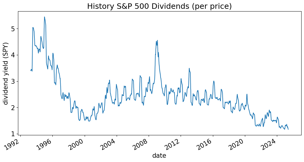
spy = pd.read_excel(INFILE,sheet_name=f'{TICKETF} history').set_index('date')
spy['EQY_DVD_YLD_IND'].rolling(21).mean().plot(title='History S&P 500 Dividends (per price)',ylabel=('dividend yield (SPY)'));
Corporate Actions#
prices = pd.read_excel(INFILE,sheet_name=f'prices {TICK}').set_index('date')

prices['Unadjusted Price'].plot(title=TICK, ylabel='price', legend=['unadjusted price']);
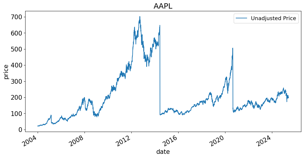
What is going on here?
Has Apple really shown so little growth since 2005?
Has Apple really crashed so hard?
dvds[dvds['dividend_type']=='Stock Split'].rename(columns={'dividend_amount':'split ratio'}).loc[:,['split ratio']].style.set_caption(f'{TICK}')
| split ratio | |
|---|---|
| record_date | |
| 2020-08-24 00:00:00 | 4.000000 |
| 2014-06-02 00:00:00 | 7.000000 |
| 2005-02-18 00:00:00 | 2.000000 |
| 2000-05-19 00:00:00 | 2.000000 |
| 1987-05-15 00:00:00 | 2.000000 |
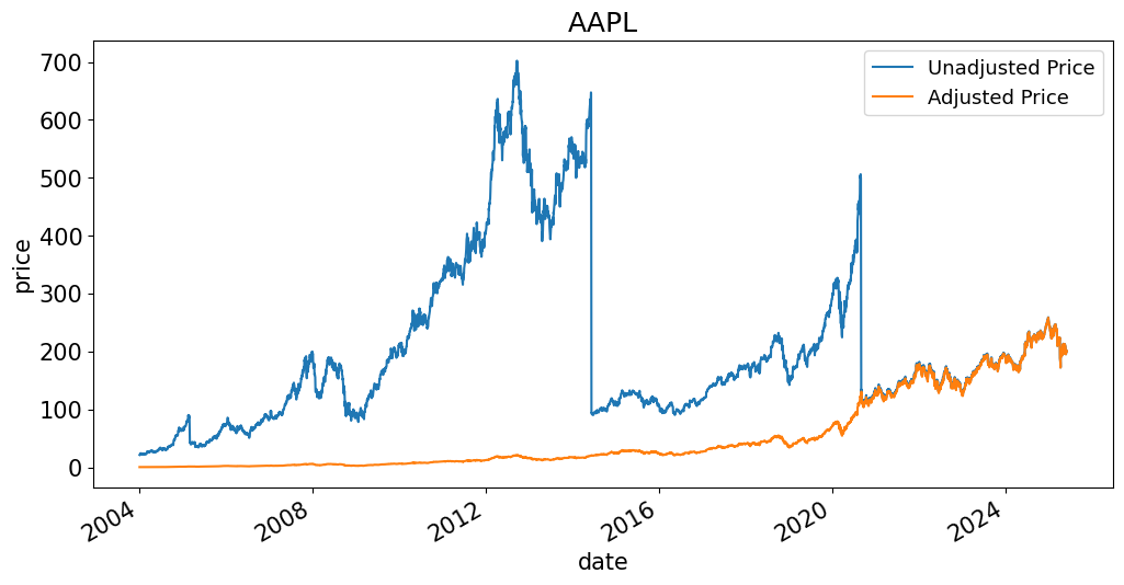
Adjusted Prices#
The adjusted price is
the same as the actual price on the final value of the timeseries.
readjusted backward through time, so earlier dates may diverge greatly
ensures a historically accurate return series can be computed
The adjusted price incorporates
regular dividends
special dividends
stock splits
prices[['Unadjusted Price','Adjusted Price']].plot(title=TICK, ylabel='price');
Technical Point: Computation of adjusted price#
Notation: \(P\): unadjusted price \(P^*\): adjusted price \(D\): dividend
We want an adjusted price series such that returns are correct, without further adjustment:
Footnote#
Adjusted prices (for dividends) are reported in a way that is slightly biased, and does not lead to a completely equivalent return on dividend days. Data providers typically calculate:
where the \(t_i\) denote the ex-dividend dates such that \(t_i > t\). Namely, each dividend causes an additional adjustment factor, \(A_i\) for all dates preceding the dividend.
The scaling is given by
However, the conversion factor needed to ensure the adjusted series gives identical returns is
In practice, this difference is very small, and everyone uses adjusted returns without worrying about this bias.
Still, if you are calculating a dividend-adjusted return by hand from the unadjusted prices, it will not quite match the price growth of the adjusted-price series.
International Stocks#
American Depository Receipts (ADR’s) are certificates traded in U.S. markets which represent foreign stocks.
ADR’s are used to make it easier for foreign firms to register securities in the U.S.
Most foreign stocks traded in U.S. markets use ADRs.
Sometimes, these are called American Depository Shares, or ADS.
SPX Sector Metrics#
Load Data#
from matplotlib.cm import get_cmap
from matplotlib import patches as mpatches
FILE_DATA = '../data/spx_metrics.xlsx'

with pd.ExcelFile(FILE_DATA) as xls:
    bdp_df = pd.read_excel(xls, sheet_name='Single Name Stats', index_col='ticker')
    sector_metrics = pd.read_excel(xls, sheet_name='Sector Stats', index_col='gics_sector_name')
    names = pd.read_excel(xls, sheet_name='Ticker Names', index_col='ticker')

# Normalize column names to lower-case
bdp_df.columns = [c.lower() for c in bdp_df.columns]
sector_metrics.columns = [c.lower() for c in sector_metrics.columns]
metrics = bdp_df.columns
# Map ticker to sector for coloring
ticker_to_sector = bdp_df['gics_sector_name']
# Prepare sector color map
sectors = sector_metrics.index.tolist()
cmap = get_cmap('tab20', len(sectors))
color_map = {s: cmap(i) for i, s in enumerate(sectors)}
/var/folders/zx/3v_qt0957xzg3nqtnkv007d00000gn/T/ipykernel_85347/605429811.py:6: MatplotlibDeprecationWarning: The get_cmap function was deprecated in Matplotlib 3.7 and will be removed in 3.11. Use ``matplotlib.colormaps[name]`` or ``matplotlib.colormaps.get_cmap()`` or ``pyplot.get_cmap()`` instead.
  cmap = get_cmap('tab20', len(sectors))
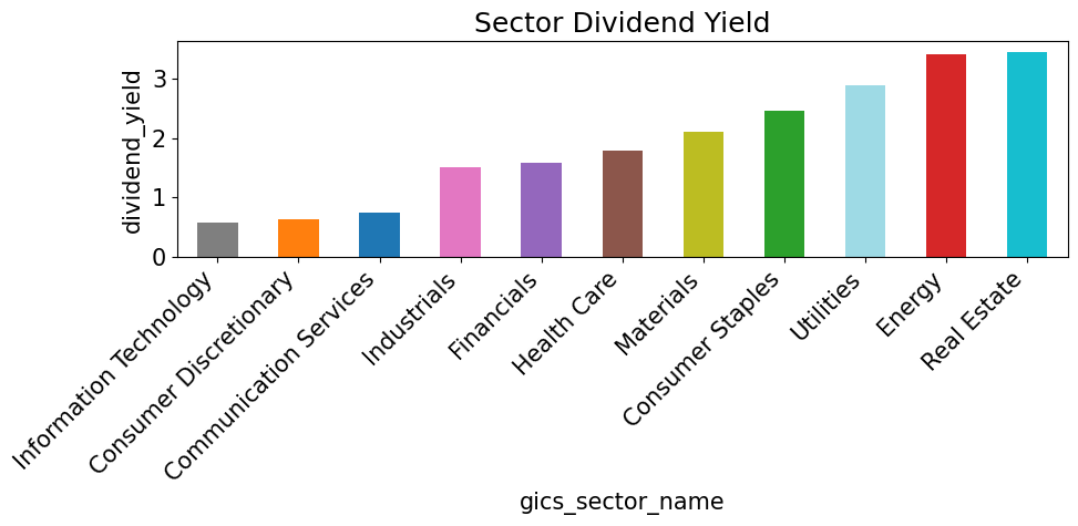
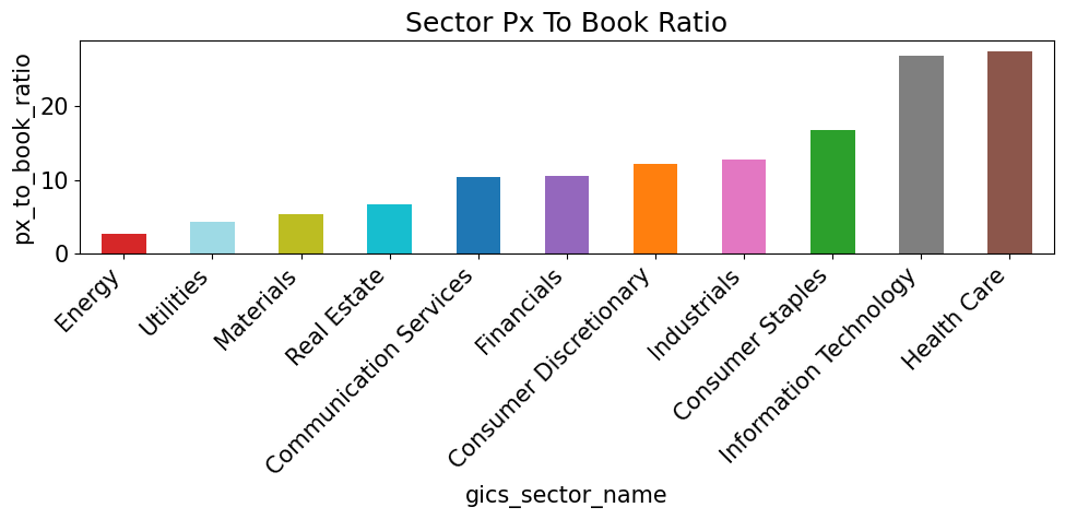
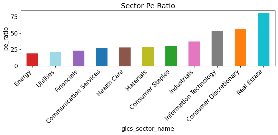
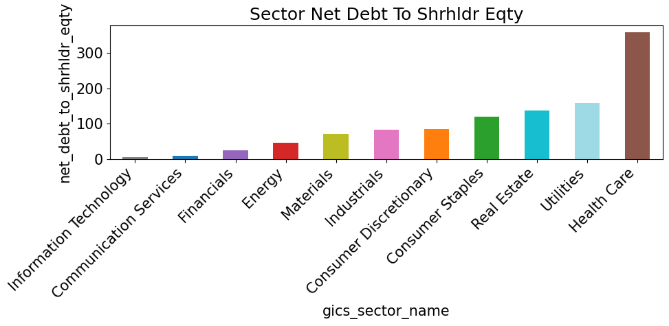
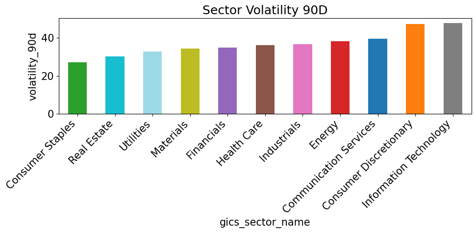
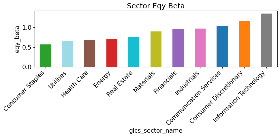
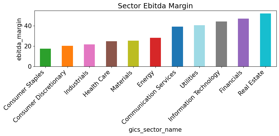
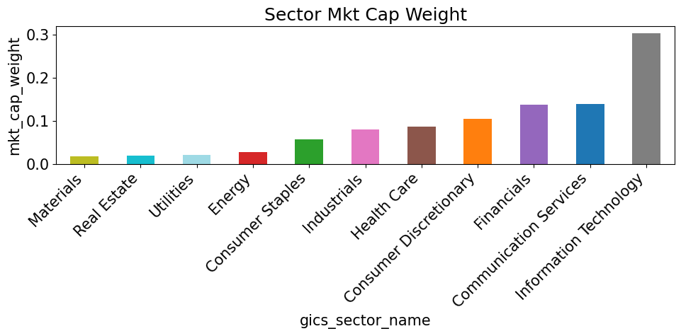
Sector Stats#
# ----------------------------------------
# PREPARE SECTOR COLOR MAP
# ----------------------------------------
sectors = sector_metrics.index.tolist()
cmap = get_cmap('tab20', len(sectors))
color_map = {s: cmap(i) for i, s in enumerate(sectors)}

# ----------------------------------------
# VISUALIZE SECTOR VARIATION
# ----------------------------------------
for metric in sector_metrics.columns:
    if metric == 'cur_mkt_cap': continue
    vals = sector_metrics[metric].sort_values()
    colors = [color_map[s] for s in vals.index]
    plt.figure(figsize=(10, 5))
    vals.plot(kind='bar', color=colors)
    plt.title(f"Sector {metric.replace('_', ' ').title()}")
    plt.ylabel(metric)
    plt.xticks(rotation=45, ha='right')
    plt.tight_layout()
    plt.show()
/var/folders/zx/3v_qt0957xzg3nqtnkv007d00000gn/T/ipykernel_85347/2578127923.py:5: MatplotlibDeprecationWarning: The get_cmap function was deprecated in Matplotlib 3.7 and will be removed in 3.11. Use ``matplotlib.colormaps[name]`` or ``matplotlib.colormaps.get_cmap()`` or ``pyplot.get_cmap()`` instead.
  cmap = get_cmap('tab20', len(sectors))
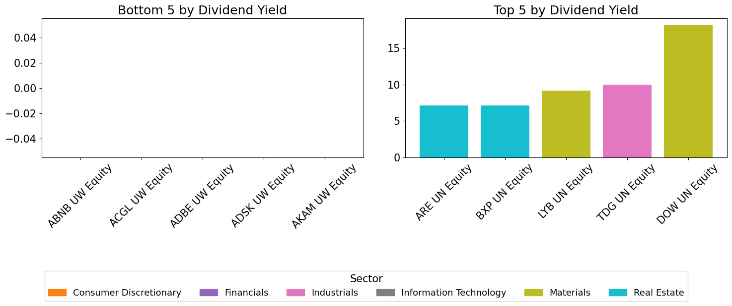
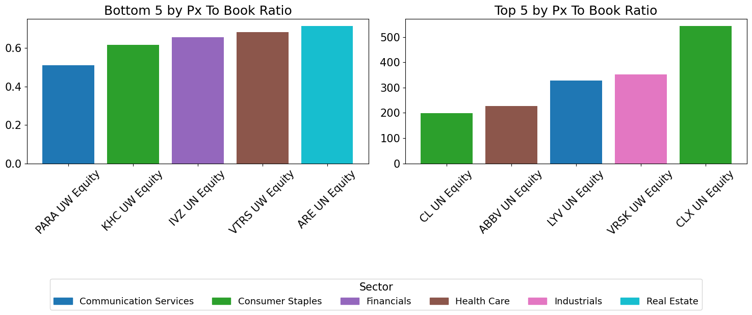
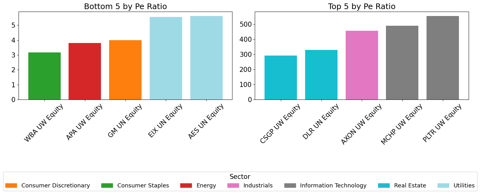
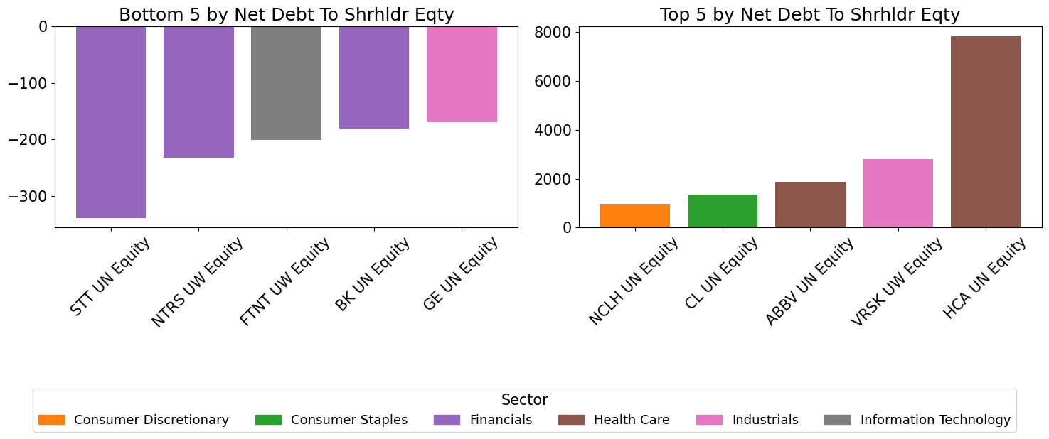
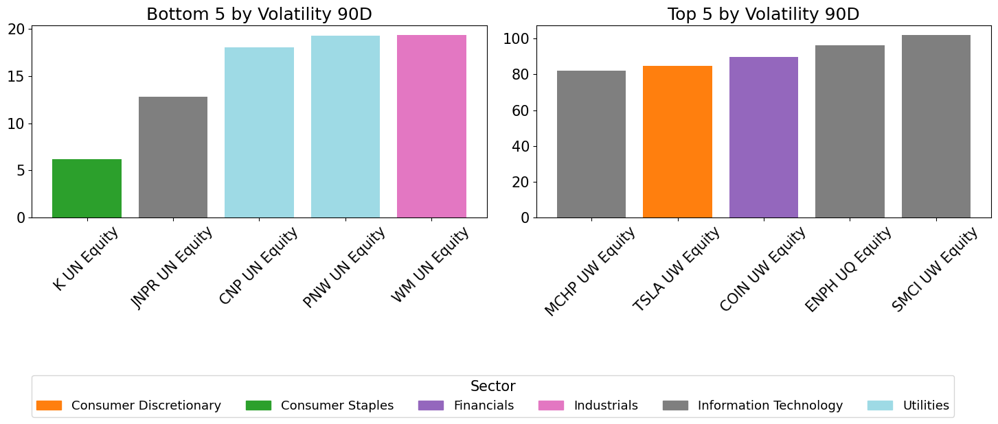
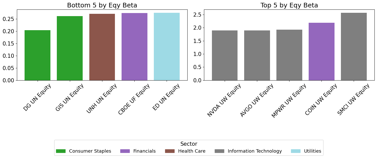
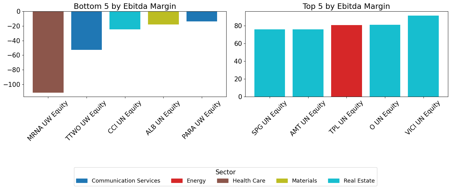
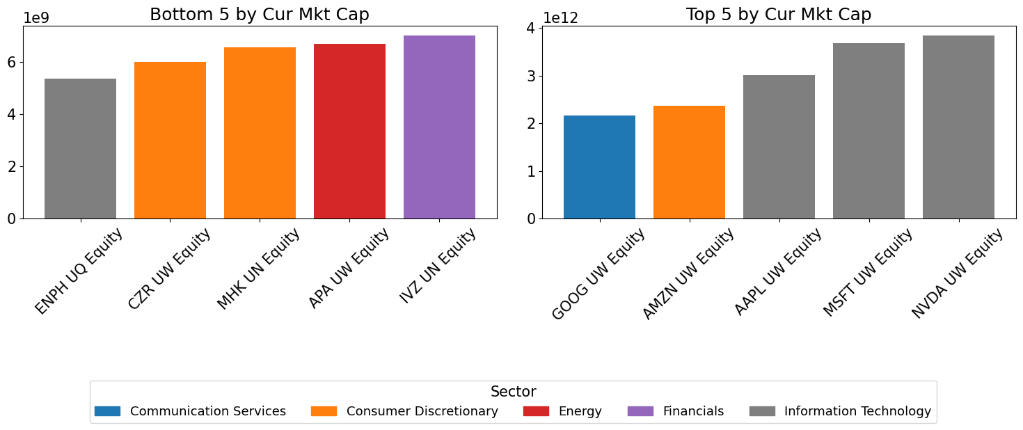
Individual Names - Highs and Lows#
# ----------------------------------------
# TOP & BOTTOM STOCKS PER METRIC
# ----------------------------------------
ticker_to_sector = bdp_df['gics_sector_name']
for m in metrics:
    if m not in bdp_df.columns: continue
    series = pd.to_numeric(bdp_df[m], errors='coerce').dropna()
    if len(series) < 2: continue
    top5 = series.nlargest(5)
    bot5 = series.nsmallest(5)
    fig, axes = plt.subplots(1, 2, figsize=(15, 5), sharey=False)
    bot = bot5.sort_values()
    axes[0].bar(bot.index, bot.values, color=[color_map[ticker_to_sector.loc[t]] for t in bot.index])
    axes[0].set_title(f"Bottom 5 by {m.replace('_', ' ').title()}")
    axes[0].tick_params(axis='x', rotation=45)
    top = top5.sort_values()
    axes[1].bar(top.index, top.values, color=[color_map[ticker_to_sector.loc[t]] for t in top.index])
    axes[1].set_title(f"Top 5 by {m.replace('_', ' ').title()}")
    axes[1].tick_params(axis='x', rotation=45)
    unique_secs = sorted({ticker_to_sector.loc[i] for i in list(bot.index)+list(top.index)})
    handles = [mpatches.Patch(color=color_map[s], label=s) for s in unique_secs]
    fig.legend(handles=handles, title='Sector', bbox_to_anchor=(0.5,-0.1), loc='upper center', ncol=len(handles))
    plt.tight_layout()
    plt.show()