Commodity Futures

import pandas as pd
import numpy as np

import seaborn as sns
import matplotlib.pyplot as plt
%matplotlib inline
plt.rcParams['figure.figsize'] = (10,5)
plt.rcParams['font.size'] = 13
plt.rcParams['legend.fontsize'] = 13

from matplotlib.ticker import (MultipleLocator,
                               FormatStrFormatter,
                               AutoMinorLocator)

LOADFILE = '../data/futures_data.xlsx'
futures_info = pd.read_excel(LOADFILE,sheet_name='futures contracts').set_index('symbol')

Definition

A futures contract is an agreement

• entered at \(t\)

• to purchase an asset at \(T\)

• for a price \(F\)

It is an obligation, not an option!

We will return to some key differences between futures and forwards.

Assets

Futures contracts are an important way to trade commodities including

• energy

• metals

• grains

• livestock

Futures contracts are traded widely on many assets beyond commodities:

• interest-rate products

• currency

• equity indexes

• other indexes

Data on Variety

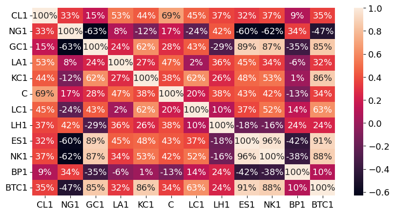
The correlation heatmap below gives a sense of the range of products.

• Most bond correlations are 80%+

• Most stock correlations are 60%+

ADJLAB = 'roll=ratio'
futures_hist = pd.read_excel(LOADFILE,sheet_name=f'continuous futures {ADJLAB}').set_index('date')
corrmat = futures_hist.loc['2015':,:].corr()
sns.heatmap(corrmat,annot=True,fmt='.0%')
plt.show()

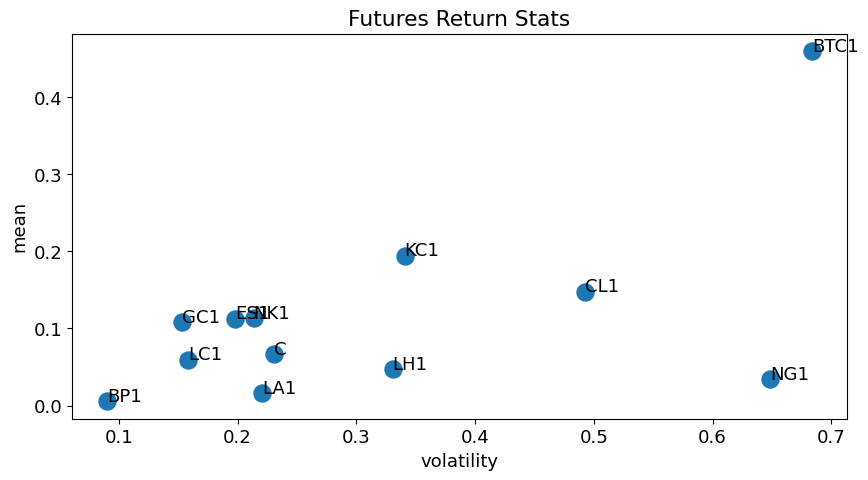
Variety of means and volatilities

px = futures_hist.copy()
px[px<0] = np.nan
rx = px.pct_change().dropna()
DAYS = rx.resample('YE').size().median()

metrics = pd.DataFrame(columns=['mean','vol'],index=rx.columns,dtype=float)
metrics['mean'] = rx.mean() * DAYS
metrics['vol'] = rx.std() * np.sqrt(DAYS)

/var/folders/zx/3v_qt0957xzg3nqtnkv007d00000gn/T/ipykernel_89789/375234581.py:3: FutureWarning: The default fill_method='pad' in DataFrame.pct_change is deprecated and will be removed in a future version. Either fill in any non-leading NA values prior to calling pct_change or specify 'fill_method=None' to not fill NA values.
  rx = px.pct_change().dropna()

df = metrics.copy().reset_index()

fig, ax = plt.subplots()
ax.scatter(x=df['vol'],y=df['mean'],s=150)
ax.set_xlabel('volatility')
ax.set_ylabel('mean')

for idx, row in df.iterrows():
    ax.annotate(row['index'], (row['vol'], row['mean']))

plt.title('Futures Return Stats')
plt.show()

Trading

Exchanges

Futures trade on exchanges. In U.S. markets, the following two exchanges are of particular note:

• Chicago Mercantile Exchange (CME)

• Intercontinental Exchange (ICE)

In recent years, the trading has moved to being overwhelmingly (and at many exchanges, completely,) electronic.

Standardization

One role of an exchange is to standardize the trading, which allows for better liquidity.

This is especially useful in commodities, to set the grade, size, location of the asset.

Clearing

As part of trading on an exchange, futures are centrally cleared. This is important for

• eliminating counterparty risk

• achieving better netting and margin requirements

Settlement

Settlement may be via

• delivery of the asset

• cash payment equal to the spot price of the asset

Note that there is cash delivery for

• equity indexes

• bitcoin (index) But there is also cash delivery for some physical assets

• Hogs are delivered via cash

• Cattle are delivered physically

futures_info[['name','category','delivery type']]

	name	category	delivery type
symbol
CL	WTI CRUDE FUTURE Jul25	Crude Oil	PHYS
NG	NATURAL GAS FUTR Jul25	Natural Gas	PHYS
GC	GOLD 100 OZ FUTR Aug25	Precious Metal	PHYS
AH	LME PRI ALUM FUTR Jun25	Base Metal	PHYS
KC	COFFEE 'C' FUTURE Sep25	Foodstuff	PHYS
ZC	CORN FUTURE Dec25	Corn	PHYS
LE	LIVE CATTLE FUTR Aug25	Livestock	PHYS
HE	LEAN HOGS FUTURE Aug25	Livestock	CASH
ES	S&P500 EMINI FUT Jun25	Equity Index	CASH
225	NIKKEI 225 (OSE) Sep25	Equity Index	CASH
6B	BP CURRENCY FUT Jun25	Currency	PHYS
BTC	CME Bitcoin Fut Jun25	Digital Assets	CASH

futures_info.style.format({
    'contract size': '{:,.0f}',
    'last_price': '{:,.2f}',
    'contract value': '{:,.0f}',
    'contract date': '{:%Y-%m-%d}',
    'margin limit': '{:,.0f}',
    'tick size': '{:,.3f}',
    'tick value': '{:,.2f}',
    'open interest': '{:,.0f}',
    'volume': '{:,.0f}',
    'volume 10d avg': '{:,.0f}',
})

	bb ticker	name	type	category	delivery type	exchange	contract date	contract size	last_price	contract value	crncy	margin limit	tick size	tick value	open interest	volume	volume 10d avg
symbol
CL	CLA Comdty	WTI CRUDE FUTURE Jul25	Physical commodity future.	Crude Oil	PHYS	New York Mercantile Exchange	2025-07-01	1,000	67.16	67,160	USD	5,206	0.010	10.00	165,870	103,983	313,670
NG	NGA Comdty	NATURAL GAS FUTR Jul25	Physical commodity future.	Natural Gas	PHYS	New York Mercantile Exchange	2025-07-01	10,000	3.60	35,980	USD	3,514	0.001	10.00	148,262	40,318	177,381
GC	GCA Comdty	GOLD 100 OZ FUTR Aug25	Physical commodity future.	Precious Metal	PHYS	Commodity Exchange, Inc.	2025-08-01	100	3,410.00	341,000	USD	15,000	0.100	10.00	319,598	130,423	184,181
AH	LAA Comdty	LME PRI ALUM FUTR Jun25	Physical commodity future.	Base Metal	PHYS	London Metal Exchange	2025-06-01	25	2,521.40	63,035	USD	nan	0.010	0.25	27,661	65,358	40,852
KC	KCA Comdty	COFFEE 'C' FUTURE Sep25	Physical commodity future.	Foodstuff	PHYS	ICE Futures US Softs	2025-09-01	37,500	348.55	130,706	USD	10,410	0.050	18.75	64,351	5,956	14,658
ZC	C A Comdty	CORN FUTURE Dec25	Physical commodity future.	Corn	PHYS	Chicago Board of Trade	2025-12-01	5,000	442.75	22,138	USD	975	0.250	12.50	516,966	13,842	111,093
LE	LCA Comdty	LIVE CATTLE FUTR Aug25	Physical commodity future.	Livestock	PHYS	Chicago Mercantile Exchange	2025-08-01	40,000	218.03	87,210	USD	2,750	0.025	10.00	164,948	26,740	28,442
HE	LHA Comdty	LEAN HOGS FUTURE Aug25	Physical commodity future.	Livestock	CASH	Chicago Mercantile Exchange	2025-08-01	40,000	110.20	44,080	USD	1,850	0.025	10.00	105,698	29,855	25,778
ES	ESA Index	S&P500 EMINI FUT Jun25	Physical index future.	Equity Index	CASH	Chicago Mercantile Exchange	2025-06-01	50	6,014.50	300,725	USD	20,174	0.250	12.50	2,056,338	207,382	1,291,841
225	NKA Index	NIKKEI 225 (OSE) Sep25	Physical index future.	Equity Index	CASH	Osaka Exchange	2025-09-01	1,000	38,050.00	38,050,000	JPY	nan	10.000	10,000.00	139,501	3,549	15,690
6B	BPA Curncy	BP CURRENCY FUT Jun25	Currency future.	Currency	PHYS	Chicago Mercantile Exchange	2025-06-01	62,500	136.13	85,081	USD	2,200	0.010	6.25	92,829	85,929	94,886
BTC	BTCA Curncy	CME Bitcoin Fut Jun25	Currency future.	Digital Assets	CASH	Chicago Mercantile Exchange	2025-06-01	5	107,265.00	536,325	USD	130,992	5.000	25.00	21,494	2,783	8,306

Quoting Conventions

https://www.cmegroup.com/markets/energy/crude-oil/light-sweet-crude.contractSpecs.html

Multiple

futures_info[['name','contract size','contract value']].style.format({'contract size':'{:,.0f}','contract value':'${:,.0f}'})

	name	contract size	contract value
symbol
CL	WTI CRUDE FUTURE Jul25	1,000	$67,160
NG	NATURAL GAS FUTR Jul25	10,000	$35,980
GC	GOLD 100 OZ FUTR Aug25	100	$341,000
AH	LME PRI ALUM FUTR Jun25	25	$63,035
KC	COFFEE 'C' FUTURE Sep25	37,500	$130,706
ZC	CORN FUTURE Dec25	5,000	$22,138
LE	LIVE CATTLE FUTR Aug25	40,000	$87,210
HE	LEAN HOGS FUTURE Aug25	40,000	$44,080
ES	S&P500 EMINI FUT Jun25	50	$300,725
225	NIKKEI 225 (OSE) Sep25	1,000	$38,050,000
6B	BP CURRENCY FUT Jun25	62,500	$85,081
BTC	CME Bitcoin Fut Jun25	5	$536,325

Tick Size

futures_info[['name','tick size','tick value']].style.format({'tick size':'{:.3f}','tick value':'{:.2f}'})

	name	tick size	tick value
symbol
CL	WTI CRUDE FUTURE Jul25	0.010	10.00
NG	NATURAL GAS FUTR Jul25	0.001	10.00
GC	GOLD 100 OZ FUTR Aug25	0.100	10.00
AH	LME PRI ALUM FUTR Jun25	0.010	0.25
KC	COFFEE 'C' FUTURE Sep25	0.050	18.75
ZC	CORN FUTURE Dec25	0.250	12.50
LE	LIVE CATTLE FUTR Aug25	0.025	10.00
HE	LEAN HOGS FUTURE Aug25	0.025	10.00
ES	S&P500 EMINI FUT Jun25	0.250	12.50
225	NIKKEI 225 (OSE) Sep25	10.000	10000.00
6B	BP CURRENCY FUT Jun25	0.010	6.25
BTC	CME Bitcoin Fut Jun25	5.000	25.00

Open Interest

Open Interest measures the number of open positions for the specific futures contract, cumulated over time.

Volume is the number of contracts traded that period (daily below).

See the chart below for the difference

futures_info[['name','open interest','volume','volume 10d avg']].style.format({'open interest':'{:,.0f}','volume':'{:,.0f}','volume 10d avg':'{:,.0f}'})

	name	open interest	volume	volume 10d avg
symbol
CL	WTI CRUDE FUTURE Jul25	165,870	103,983	313,670
NG	NATURAL GAS FUTR Jul25	148,262	40,318	177,381
GC	GOLD 100 OZ FUTR Aug25	319,598	130,423	184,181
AH	LME PRI ALUM FUTR Jun25	27,661	65,358	40,852
KC	COFFEE 'C' FUTURE Sep25	64,351	5,956	14,658
ZC	CORN FUTURE Dec25	516,966	13,842	111,093
LE	LIVE CATTLE FUTR Aug25	164,948	26,740	28,442
HE	LEAN HOGS FUTURE Aug25	105,698	29,855	25,778
ES	S&P500 EMINI FUT Jun25	2,056,338	207,382	1,291,841
225	NIKKEI 225 (OSE) Sep25	139,501	3,549	15,690
6B	BP CURRENCY FUT Jun25	92,829	85,929	94,886
BTC	CME Bitcoin Fut Jun25	21,494	2,783	8,306

Closing Positions

Most open interest is ultimately closed via offsetting contracts, NOT delivery.

Consider the open interest for various contracts on Crude Oil (CL) and Gold (GC).

For each contract, we see the open interest rises about a month before the delivery, and then drops to nearly zero just before delivery.

TICKS = ['CL','GC']

futures_ts = pd.read_excel(LOADFILE,sheet_name='futures timeseries',header=[0,1,2]).droplevel(2,axis=1)
futures_ts.set_index(futures_ts.columns[0],inplace=True)
futures_ts.index.name = 'date'
futures_ts = futures_ts.swaplevel(axis=1)

idx = 0
exname = futures_ts['OPEN_INT'].iloc[:,idx].name
exdata = futures_ts['OPEN_INT'].iloc[:,idx].dropna()
exdata.plot(title=f'Open Interest for {exname}');

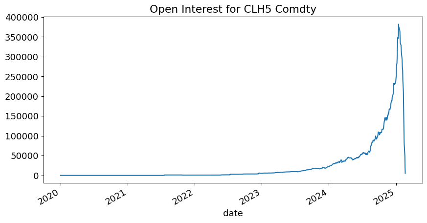
intpct = exdata[-1]/exdata.max()
print(f'Open Interest at close is {intpct:.2%} of its peak!')

Open Interest at close is 1.40% of its peak!

/var/folders/zx/3v_qt0957xzg3nqtnkv007d00000gn/T/ipykernel_89789/2823046234.py:1: FutureWarning: Series.__getitem__ treating keys as positions is deprecated. In a future version, integer keys will always be treated as labels (consistent with DataFrame behavior). To access a value by position, use `ser.iloc[pos]`
  intpct = exdata[-1]/exdata.max()

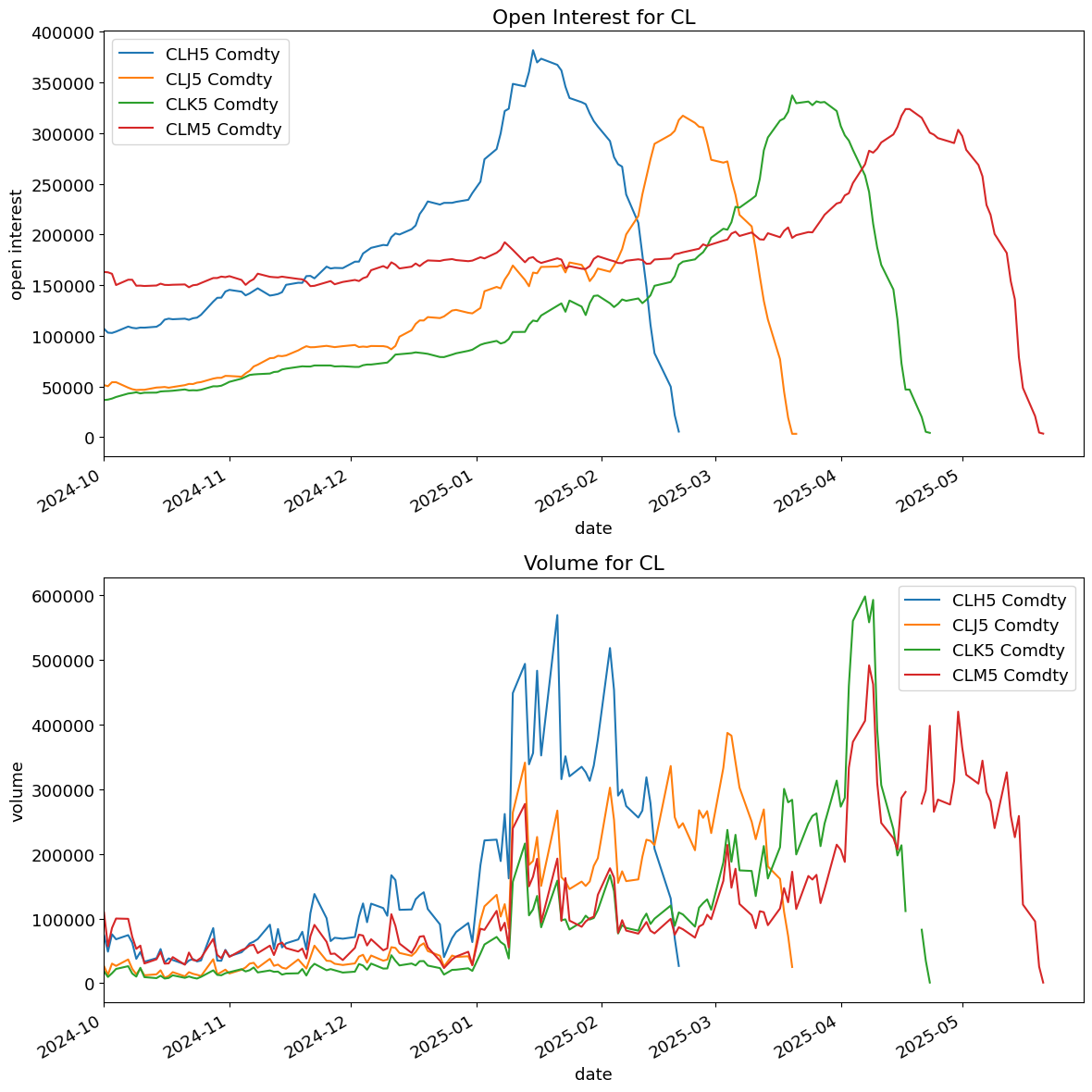
Active Contract

For a given futures chain, only a few are liquid.

The active contract is typically denoted as the front-month (nearest expiration) which typically corresponds with the contract with the highest open interest.

For the two examples below, we see that the soonest-to-expiry sees a spike in open interest, with the second-nearest expiry rising in anticipation of being the active contract.

Liquidity

Thus, the active contract tends to be much more liquid , as measured by volume or open interest.

As a corollary, a contract will be listed, yet may receive almost zero interest or volume for months or years.

In the example above, note that the open interest is miniscule for a year.

PLOTDATESTART = '2024-10'
PLOTDATEEND = '2025-05-31'

fig, ax = plt.subplots(2,1,figsize=(12,12))
futures_ts['OPEN_INT'].iloc[:,0:4].plot(ax=ax[0],xlim=(PLOTDATESTART,PLOTDATEEND),title=f'Open Interest for {TICKS[0]}',ylabel='open interest')
futures_ts['VOLUME'].iloc[:,0:4].plot(ax=ax[1],xlim=(PLOTDATESTART,PLOTDATEEND),title=f'Volume for {TICKS[0]}',ylabel='volume')
plt.tight_layout()
plt.show()

Margins and Marking to Market

marg = futures_info[['name']].copy()
marg['margin limit %'] = futures_info['margin limit']/futures_info['contract value']

marg['vol'] = rx.std().values
marg['margin sigma'] = marg['margin limit %'] / marg['vol']
marg.set_index('name',inplace=True)
marg.index = [' '.join(row.split()[:-2]) for row in marg.index]

marg.dropna().sort_values('margin sigma').style.format({'margin limit %':'{:.1%}','vol':'{:.1%}','margin sigma':'{:.1f}'})

	margin limit %	vol	margin sigma
LEAN HOGS	4.2%	2.0%	2.0
NATURAL GAS	9.8%	4.0%	2.4
WTI CRUDE	7.8%	3.1%	2.5
CORN	4.4%	1.4%	3.1
LIVE CATTLE	3.2%	1.0%	3.2
COFFEE 'C'	8.0%	2.1%	3.8
BP CURRENCY	2.6%	0.6%	4.6
GOLD 100 OZ	4.4%	1.0%	4.6
S&P500 EMINI	6.7%	1.2%	5.5
CME Bitcoin	24.4%	4.2%	5.8

Futures References

The CME provides a helpful series of videos for an introduction to Futures

https://www.cmegroup.com/education/courses/introduction-to-futures/definition-of-a-futures-contract.html

Pricing

Forward Price

The basic model of a futures price is:

\[F_0 = S_0 e^{r_f T}\]

This equation is derived by no-arbitrage, in a simplified setting of

• no market frictions

• a constant risk-free rate, \(r_f\)

• no financing considerations (margin, marking to market, etc)

This is just the forward pricing equation.

It says that the futures price should be the spot price compounded by the risk-free rate until delivery.

Carry

The pricing formula above accounts for the time-value of money, but it does not account for the carry cost of the asset.

Dividend yield

Suppose that the asset pays a dividend yield of \(q\)

• dividends on stock index

• lease rate on metals

Storage cost

The asset may be costly to store, such that it has a negative carry.

• oil, grains, etc

Carry

Let carry, \(c\), denote the net difference of the storage costs minus income.

Then,

\[F_0 = S_0 e^{(r_f+c)T}\]

That is, the

• higher the storage costs, the higher the futures price.

• higher the income, the lower the futures price.

Convenience Yield

For consumption assets, the no-arbitrage argument is more complicated.

\[F_0 < S_0e^{(r_f+c)T}\]

This is due to the fact that the asset has a convenience yield, \(y\).

This convenience yield is not explicit income to the owner, but rather potential income should the consumption use of the asset be important during the contract period.

The equation can make explicit note of this,

\[F_0 = S_0e^{(r_f+c-y)T}\]

or simply include the convenience yield as part of the carry.

\[F_0 = S_0e^{(r_f+c^*)T}\]

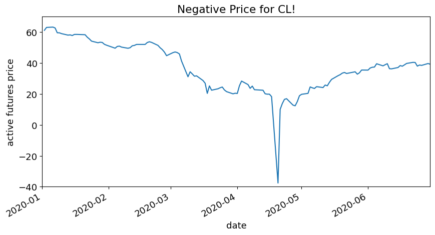
Negative Price for Oil?

Typically, carry costs are a second-order factor for prices.

But sometimes market frictions cause them to be of high importance.

TICK = 'CL'
data_comp = pd.read_excel(LOADFILE,sheet_name=f'roll conventions {TICK}',header=[0,1,2]).droplevel(2,axis=1)
data_comp.set_index(data_comp.columns[0],inplace=True)
data_comp.index.name = 'date'
data_comp = data_comp.swaplevel(axis=1).droplevel(0,axis=1)
data_comp['CL1 Comdty'].plot(xlim=('2020-01-01','2020-06-30'),ylim=(-40,70),title=f'Negative Price for {TICK}!',ylabel='active futures price');

References

https://www.nytimes.com/2020/04/20/business/oil-prices.html https://www.forbes.com/sites/sarahhansen/2020/04/21/heres-what-negative-oil-prices-really-mean/?sh=5530d0185a85

Complications

There are various complications to the simple model.

Moving Interest Rates

The formulas above assume a constant interest rate.

If the interest rate moves, then we would have the following adjustments:

• Higher price if asset is positively correlated to the asset value

• Lower price if asset is negatively correlated to the asset value Why?

Daily Settlement

Futures contracts are settled daily, which means the cashflows are paid/received day-by-day rather than all at delivery.

Terminology

• Daily Settlement: The profit/loss of the day is settled via an accrual / deduction from the margin account. This payment is irrevocable. That is to say that it is not collateral but a permanent payment based on the day’s movement.

• Variation Margin: To reduce counterparty risk in some collateralized trades, (such as repo,) you might need to pay a variation margin when the collateral value goes down. This is a form of collateral: it earns interest on your behalf, and it will be returned at the end of the trade.

• Mark-to-market: Revising the price of an asset in the financial records, (such as a balance sheet,) to reflect the market movements in the price. This has no implications for cashflow but rather is a financial accounting revision. This term is often used to refer to teh daily settlement mentioned above, but this term is more general.

Futures vs Forwards

The CME video compares and contrasts.

https://www.cmegroup.com/education/courses/introduction-to-futures/futures-contracts-compared-to-forwards.html

• For each difference, would it cause the price of the future contract to be more or less than the comparable forward?

• Which differences do you think are of most practical importance?

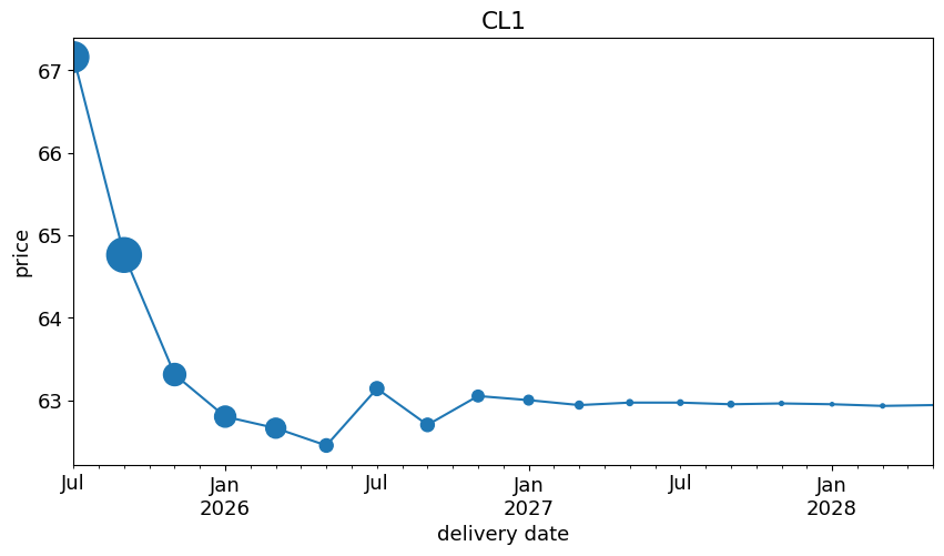
The Futures Curve

Defining the Curve

At a given date, consider the full chain of some futures contract:

list_curves = ['CL1','GC1']
curves = dict()
for comdty in list_curves:
    curves[comdty]= pd.read_excel(LOADFILE,sheet_name=f'curve {comdty}')

curves[comdty].style.format({'price':'${:,.2f}', 'open interest':'{:,.0f}','deliver date':'{:%Y-%m-%d}'})

	ticker	delivery date	price	open interest
0	GCM5 Comdty	2025-06-02 00:00:00	$3,387.10	1,828
1	GCQ5 Comdty	2025-08-01 00:00:00	$3,409.50	319,598
2	GCV5 Comdty	2025-10-01 00:00:00	$3,435.00	20,568
3	GCZ5 Comdty	2025-12-01 00:00:00	$3,465.80	61,091
4	GCG6 Comdty	2026-02-02 00:00:00	$3,489.90	9,796
5	GCJ6 Comdty	2026-04-01 00:00:00	$3,466.40	2,560
6	GCM6 Comdty	2026-06-01 00:00:00	$3,520.90	529
7	GCQ6 Comdty	2026-08-03 00:00:00	$3,550.70	85
8	GCV6 Comdty	2026-10-01 00:00:00	$3,520.10	13
9	GCZ6 Comdty	2026-12-01 00:00:00	$3,595.00	78

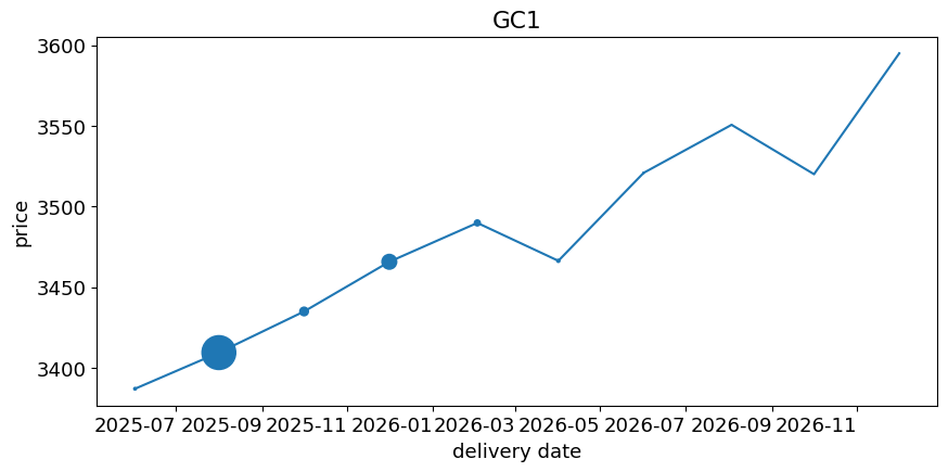
If we plot this chain against the delivery dates, we get the futures curve.

The curves below show the marker sizes in proportion to the open interest of each contract.

for comdty in list_curves:
    
    temp = curves[comdty].set_index('delivery date').sort_index()
    msize = (temp['open interest']/temp['open interest'].max()) * 500
    
    fig, ax=plt.subplots()
    temp['price'].plot(ax=ax,marker=None,title=comdty)
    temp.reset_index().plot.scatter('delivery date','price',s=msize,ax=ax,title=comdty)
    plt.show()

Backwardation and Contango

Relative to expectations

“Normal” Backwardation

• the futures price is below the expected future spot

Contango

• the futures price is above the expected future spot

Economics

Normal?

“Normal” backwardation refers to economists (Keynes) thinking it should be the “normal” situation to have the futures price below the expected future spot.

The argument depends on the assumption that hedgers (suppliers) would tend to be short the futures contract while market-makers and speculators would be long. The risk aversion of the former group being higher than the latter group might lead to the futures price being pressured below the market forecast

Relation to pricing equations above

The simple pricing above implies…

• Contango = high carry costs relative to convenience yield

• Backwardation = low carry costs relative to convenience yield

Descriptions of the futures curve

Note that

• there is not an objective “expected future spot”.

• thus, whether in backwardation or contango would depend on one’s model of the forecasted spot price.

In practice, these terms are often used with the assumption that today’s spot is the best prediction of the future spot:

\(\begin{align} P_t = \boldsymbol{E}_t\left[P_T\right] \end{align}\)

Common usage

This leads to the common usage.

Backwardation

• the futures curve is downward sloping

Contango

• the futures curve is upward sloping

This definition is simpler and can be directly measured.

In the examples above

• Oil is in backwardation

• Gold is in contango

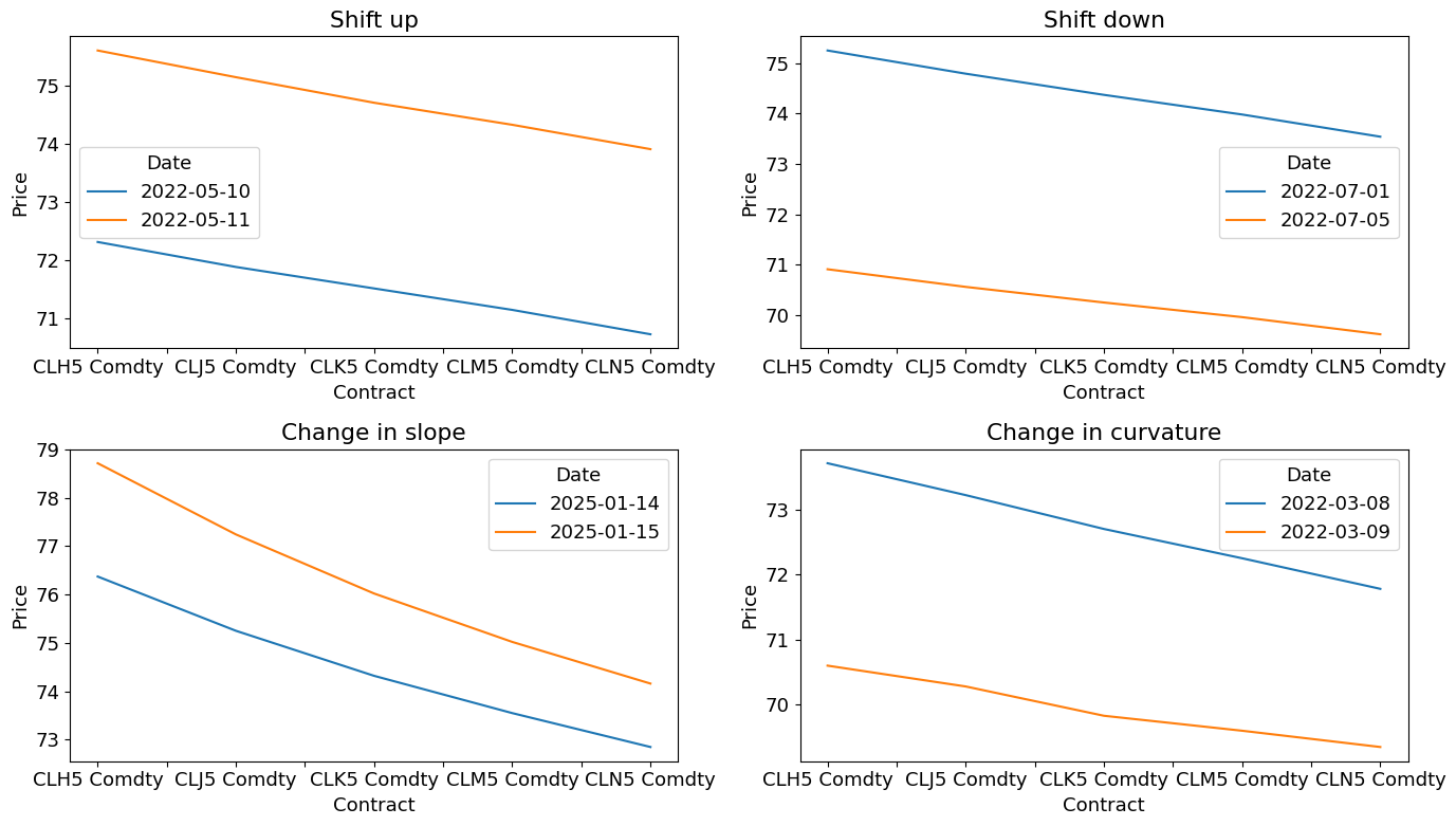
Does Backwardation Guarantee a Profit?

df = pd.read_excel(
    LOADFILE,
    sheet_name="futures timeseries",
    header=[0, 1],
    index_col=0,         # first column → index
    parse_dates=[0],     # parse that same column as dates
)
df_px_last    = df.xs("LAST_PRICE", axis=1, level=1)
px_curves = df_px_last.loc[:, df_px_last.columns.str.startswith("CL")].dropna()

slopes = px_curves.diff(axis=1)
slope_range = slopes.max(axis=1) - slopes.min(axis=1)
curvature = slopes.diff(axis=1)
curv_range = curvature.max(axis=1) - curvature.min(axis=1)

idx_list = []
idx_list.append(px_curves.diff().mean(axis=1).idxmax())
idx_list.append(px_curves.diff().mean(axis=1).idxmin())
idx_list.append(slope_range.abs().idxmax())
idx_list.append(curv_range.abs().idxmax())

import matplotlib.pyplot as plt
import pandas as pd

list_titles = ['Shift up', 'Shift down', 'Change in slope', 'Change in curvature']
fig, axes = plt.subplots(2, 2, figsize=(14, 8))

for ax, idx in zip(axes.flatten(), idx_list):
    prev_date = df.index[df.index < idx].max()
    # plot (legend will pick up the raw datetime strings)
    px_curves.loc[prev_date:idx].T.plot(ax=ax)

    # grab the handles & labels, then reformat the labels
    handles, labels = ax.get_legend_handles_labels()
    new_labels = [pd.to_datetime(lbl).strftime("%Y-%m-%d") for lbl in labels]
    ax.legend(handles, new_labels, title="Date")

    ax.set_title(list_titles[0])
    list_titles.pop(0)
    ax.set_xlabel("Contract")
    ax.set_ylabel("Price")

plt.tight_layout()
plt.show()

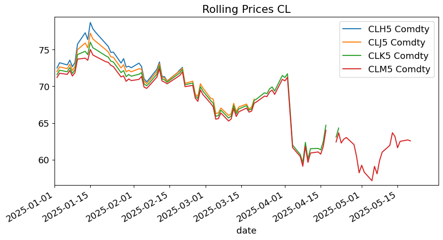
Roll

Trading futures positions involves rolling the position to new contracts.

If the curve is in contango this rolling will require buying at a higher price

• add capital to hold same number of contracts

• keep capital flat, but in fewer contracts

If the curve is in backwardation this rolling will mean buying at a lower price

• reallocate some capital to hold same number of contracts

• keep capital flat, but in more contracts

The chart below shows price histories for various contracts on the chain, note that when one settles, a trader would have to roll up/down to another contract.

PLOTDATESTART_2 = '2025-01'

ptitle = futures_ts['LAST_PRICE'].iloc[:,0].name[:2]
temp = futures_ts['LAST_PRICE'].iloc[:,0:4][PLOTDATESTART_2:PLOTDATEEND]
temp.plot(xlim=(PLOTDATESTART_2,PLOTDATEEND),ylim=(.99*temp.min().min(),1.01*temp.max().max()),title=f'Rolling Prices {ptitle}');

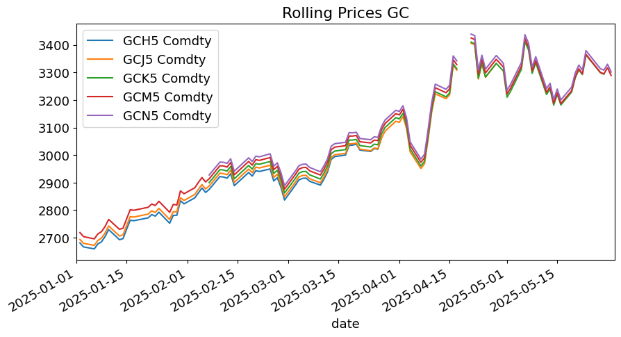
ptitle = futures_ts['LAST_PRICE'].iloc[:,-1].name[:2]
temp = futures_ts['LAST_PRICE'].iloc[:,5:][PLOTDATESTART_2:PLOTDATEEND]
temp.plot(xlim=(PLOTDATESTART_2,PLOTDATEEND),title=f'Rolling Prices {ptitle}');

Continuous Contract

Given that futures contracts mature and roll off, it can be a challenge to obtain a long history of their prices.

This is similar to getting long timeseries of bond prices.

Generic indexes

Like with bonds, the answer is to construct a generic index which is the compilation of many short-term instruments.

With bonds, this is done by building so-called “constant maturity” series, which at any point in the past point might point to the bonds closest in maturity to the stated index.

For futures, an index can be constructed by simply pointing to the active contract at any point in time.

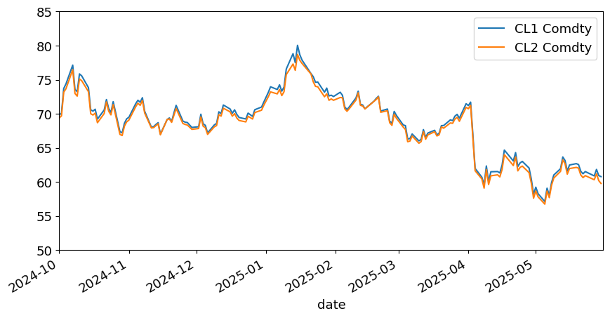
Generic front and back

The common notation is to denote the generic front contract with a “1” and the generic back contract with a “2”.

For example, for crude oil, (CL), we have

• CL1

• CL2

The chart below shows these price series.

data_comp[['CL1 Comdty','CL2 Comdty']].plot(xlim=(PLOTDATESTART,PLOTDATEEND),ylim=(50,85));

Rolling the Continuous Series

The complication with the continuous front and back futures series is that at the time of rolling, the price will jump simply due to the roll.

In analyzing the series, it will seem that these jumps are returns, when they are actually just a rebasing of the contract.

If a series tends to be in contango, this will make the returns seem artificially high.

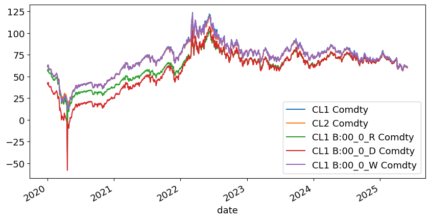
Adjusting the Continuous Series

To avoid these jumps in the series, it is common to see one of three adjustments made at each roll, going back through time, to keep the breaks continuous.

• difference: adjust the level by an addititive factor

• ratio: adjust the past series by a multiplicative factor

• weighted average: roll between the front and back contracts over a window of \(m\) days, taking a weighted average between the contracts.

The effect of all three adjustments is to

• eliminate jumps at roll dates.

• report true historic prices for the most recent contract used in the continuous series

• report an adjusted price for the earlier contracts used in the continuous series

In these ways, it is similar to the adjustments to equity prices discussed in another note.

So which adjustment to use?

• difference: keeps the profit and loss true, which is useful if simulating a particular number of contracts

• ratio: ensures valid return series, which is useful if simulating a particular investment size.

data_comp.plot();

Roll Rule

There is also a decision to make regarding when to roll the contract in the continuous series. The most popular rules are

• fixed date (often first day of the month)

• at contract close

• when the max open interest shifts

Careful with the roll method

Using an improper roll method for historic analysis may greatly misrepresent the performance.

Which of these is correct for understanding returns over time?

px = data_comp.copy()
px[px<0] = np.nan
px[px==np.inf] = np.nan
rx_comp = px.pct_change()

metrics_comp = pd.DataFrame(columns=['mean','vol'],index=rx_comp.columns,dtype=float)
metrics_comp['mean'] = rx_comp.mean() * DAYS
metrics_comp['vol'] = rx_comp.std() * np.sqrt(DAYS)
metrics_comp.iloc[:3,:].style.format('{:.1%}')

/var/folders/zx/3v_qt0957xzg3nqtnkv007d00000gn/T/ipykernel_89789/1016369827.py:4: FutureWarning: The default fill_method='pad' in DataFrame.pct_change is deprecated and will be removed in a future version. Either fill in any non-leading NA values prior to calling pct_change or specify 'fill_method=None' to not fill NA values.
  rx_comp = px.pct_change()

	mean	vol
CL1 Comdty	16.8%	57.0%
CL2 Comdty	17.0%	60.7%
CL1 B:00_0_R Comdty	17.6%	55.2%