Yields

import pandas as pd
import numpy as np

import matplotlib.pyplot as plt
%matplotlib inline
plt.rcParams['figure.figsize'] = (12,6)
plt.rcParams['font.size'] = 15
plt.rcParams['legend.fontsize'] = 13

from cmds.treasury_cmds import compound_rate, intrate_to_discount

Data Source

CRSP Treasury Monthly Release accessed via WRDS

For any given date, obtain quotes for nearly every issued Treasury.

In particular,

• Bills, Notes, Bonds

• TIPS

In the analysis below, we exclude TIPS to focus on nominal rates.

The data set does not include Floating Rate Notes (FRNs).

QUOTE_DATE = '2024-04-30'

filepath_rawdata = f'../data/treasury_quotes_{QUOTE_DATE}.xlsx'
data = pd.read_excel(filepath_rawdata,sheet_name='quotes').set_index('KYTREASNO')

Yield to Maturity (YTM) and Returns

The formula for YTM looks like the pricing formula for a bond, but replacing the maturity-dependent discount rate with a constant discount rate:

Definition

Let \(P_j(t,T,c)\) denote the price of

• bond \(j\)

• observed time-\(t\)

• which matures at time \(T\)

• with coupons occuring at interim cashflow dates \(T_i\) for \(1\le i <n\)

• and a final coupon and principal payment occuring at maturity \(T\).

Define the yield-to-maturity for bond \(j\) as the term \(y_j\) which satisfies the following equation:

\[\begin{align} P_j(t,T,c) = \sum_{i=1}^{n-1}\frac{100\left(\frac{c}{2}\right)}{\left(1+\frac{y_j}{2}\right)^{2(T_i-t)}} + \frac{100\left(1+\frac{c}{2}\right)}{\left(1+\frac{y_j}{2}\right)^{2(T-t)}} \end{align} \]

Note that the same rate, \(y_j\), is discounting cashflows at different maturities.

• It is unique to the security, \(j\).

• It is constant across the security’s various cashflow maturities.

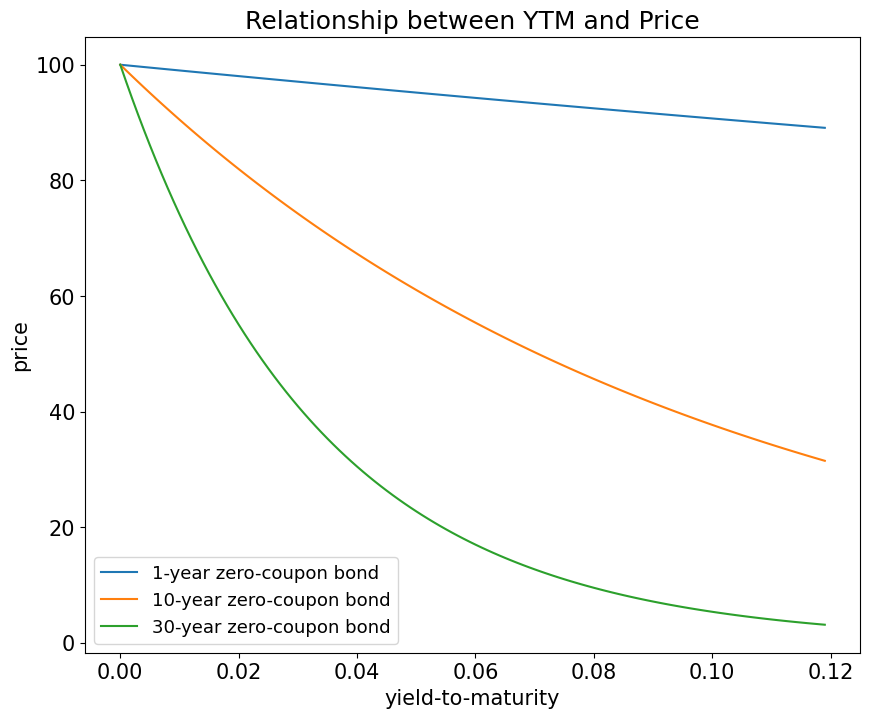
YTM has a nonlinear and inverse relationship with price

ylds_grid = np.arange(0,.12,.001)
T_grid = [1,10,30]
price_grid = pd.DataFrame(data=np.zeros([len(ylds_grid),len(T_grid)]), index=ylds_grid, columns=T_grid)
for T in T_grid:
    for i,y in enumerate(ylds_grid):
        price_grid.loc[y,T] = 100/(1+y/2)**(2*T)

price_grid.plot(figsize=(10,8))

legend_labels = [''] * len(T_grid)
for i,T in enumerate(T_grid):
    legend_labels[i] = f'{T}-year zero-coupon bond'

plt.xlabel('yield-to-maturity')
plt.ylabel('price')
plt.legend(legend_labels)
plt.title('Relationship between YTM and Price')
plt.show()

YTM will differ across coupon rates, even for the same maturity

# find maturity where YTM differs by large amount
temp = data.pivot_table(index='maturity date',values='ytm',aggfunc={'ytm':np.ptp}).sort_values('ytm',ascending=False)
# restrict answer to maturity greater than one year, to avoid short-term liquidity explanations
idx = temp[temp.index >'2024-01-01'].index[0]

tab = data[data['maturity date']==idx]

tab[['type','quote date','issue date','maturity date','ttm','cpn rate','price','ytm','total size']].style.format(
    {'ytm':'{:.3%}',
    'issue date': '{:%Y-%m-%d}', 
    'quote date': '{:%Y-%m-%d}', 
    'maturity date': '{:%Y-%m-%d}',                                                                                                                             
    'price':'{:.2f}', 
    'cpn rate':'{:.2f}', 
    'ttm':'{:.2f}', 
    'ask-bid':'{:.2f}',
    'total size':'{:.1e}'
    })

	type	quote date	issue date	maturity date	ttm	cpn rate	price	ytm	total size
KYTREASNO
207844	note	2024-04-30	2022-02-15	2025-02-15	0.80	1.50	97.03	5.347%	8.0e+10
206825	note	2024-04-30	2015-02-15	2025-02-15	0.80	2.00	97.41	5.358%	6.6e+10
204084	bond	2024-04-30	1995-02-15	2025-02-15	0.80	7.62	102.09	4.883%	9.5e+09

Returns

The return on a bond between \(t\) and \(T\) is, like any security, the (time \(T\)) payoff divided by the (time \(t\)) price.

\[ \begin{align} \left(\frac{\text{payoff}_T}{\text{investment}_t}\right)^{\frac{1}{T-t}} - 1 \end{align} \]

Note that the exponent \(1/(T-t)\) is to annualize the return.

Conditions where return equals YTM

The return to a bond is typically NOT the same as its YTM

They are only equivalent if…

1. We are discussing a zero-coupon bond. (ie It only pays cashflow at maturity.)

2. The investor holds it until maturity.

YTM vs Return for a Coupon Bond

For a coupon bond, YTM is not the same as return, whether or not the bond is held to maturity.

YTM is the exact same as Internal Rate of Return in Corporate Finance

• YTM is a discount rate that varies by instrument but is constant across the instrument’s cashflow.

• It is NOT the return, as there is no guarantee you can reinvest intermediate cashflows at the YTM.

• YTM only exists and is uniquely defined for cashflows that have the typical pattern.

YTM is just an alternate way to quote a price

• Prices for coupon bonds have a wide range due to coupons and maturity.

• YTM is a narrower range which (partially) adjusts for the time-value of money

The Yield Curve

The yield curve plots the yields against time-to-maturity.

Examine this with the ytm of every outstanding treasury issue.

data.set_index('ttm')['ytm'].plot(linestyle='',marker='*', color='k')
plt.legend()
plt.xlabel('years-to-maturity')
plt.ylabel('yield')
plt.title('Yield Curve')
plt.show()

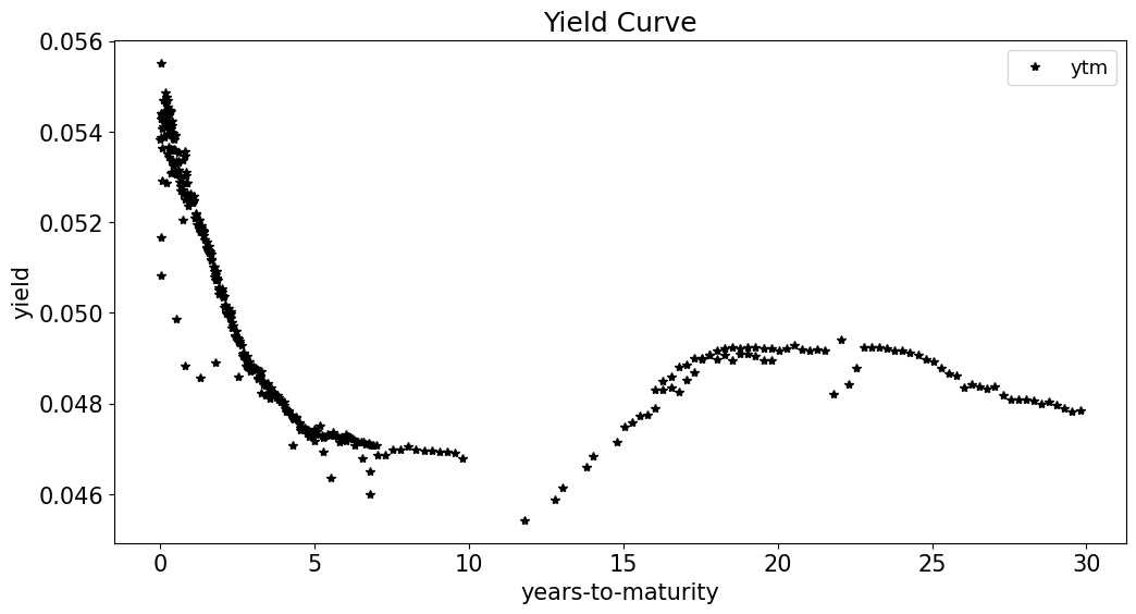
It’s not exactly a curve!

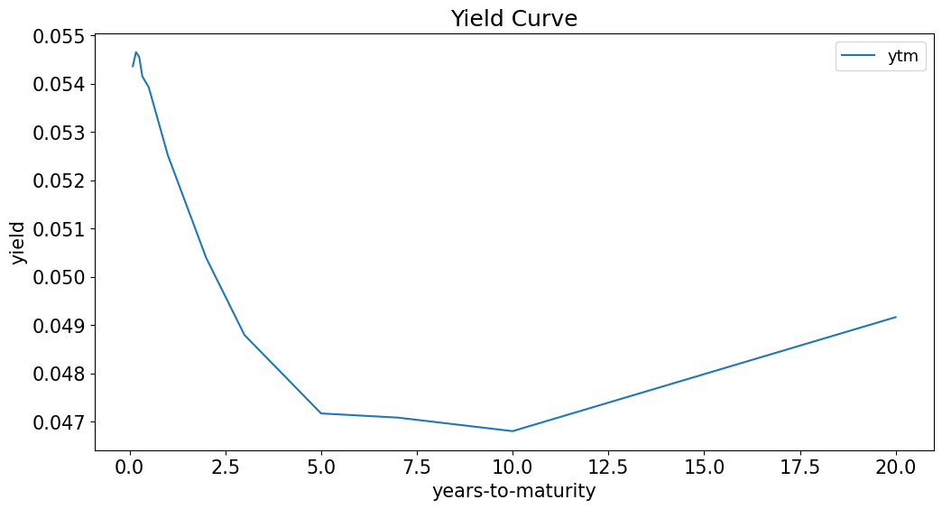
Models of the Yield Curve

The Treasury publishes constant maturity benchmarks:

https://home.treasury.gov/resource-center/data-chart-center/interest-rates/TextView?type=daily_treasury_yield_curve&field_tdr_date_value_month=202406

The Fed discusses curve-fitting of the yields here:

https://www.federalreserve.gov/data/yield-curve-models.htm

mats = [1/12,2/12,3/12,4/12,6/12,1,2,3,5,7,10,20,30]

ycurve_key = pd.DataFrame(dtype=float,index=mats,columns=['ytm'])
for mat in mats:
    idx = (data['ttm']-mat).abs().idxmin()
    ycurve_key.loc[mat,'ytm'] = data.loc[idx,'ytm']

ycurve_key.plot()

plt.legend()
plt.xlabel('years-to-maturity')
plt.ylabel('yield')
plt.title('Yield Curve')
plt.show()

---

Appendix: Compounding

Compounding

Note that the spot rate above, \(r(t,T_i)\) was applied semiannually. This was chosen for convenience with the semiannual coupons.

We could compound these spot rates to any frequency, including a continuously compounded rate.

When emphasizing the compounding chosen for the spot rate, we will subscript it by \(n\).

n	compounding frequency
1	annual
2	semiannual
4	quarterly
12	monthly
52	weekly
365	daily
\(\infty\)	continuous

For instance, changing the compounding from semiannually to daily would be,

\[ \begin{align} r_{365} = 365\left[\left(1+\frac{r_2}{2}\right)^{\frac{2}{365}}-1\right] \end{align} \]

Continuous compounding is often most useful

Because the continuously compounded rate is so useful and used so often rather than use \(r_n\) we will drop the subscript entirely and just use \(r\) with no subscript instead.

The continuously compounded rate \(r\) can be written as a function of the \(n\)-times compounded rate as follows.

\[\begin{split} \begin{align} \displaystyle r &= n\ln\left(1+\frac{r_n}{n}\right)\\ \displaystyle r_n&= n\left(e^{\frac{r}{n}}-1\right) \end{align} \end{split}\]

Discount is equivalent for any compounded rate

Note that all the compounded rates will imply the same discount, when the compounding frequency is accounted for.

\(\displaystyle\text{discount} \equiv \; Z(t,T) = \frac{1}{\left(1+\frac{r_n}{n}\right)^{n(T-t)}} \; = e^{-r(T-t)}\)

Example

Consider, as an example, the annually compounded spot rate of 5% at a maturity of \(T-t=1\).

rate = .05
compound_base = 1

ngrid = [1, 2, 4, 12, 52, 365]
compounded_rate = pd.DataFrame(index=ngrid,columns=['rate','discount'],dtype=float)
for n in ngrid:
    compounded_rate.loc[n] = compound_rate(rate,compound_base,n)
    compounded_rate.loc[n,'discount'] = 1/(1+compounded_rate.loc[n,'rate']/n)**n
    
compounded_rate.loc['continuous','rate'] = compound_rate(rate,compound_base,None)
compounded_rate.loc['continuous','discount'] = intrate_to_discount(compounded_rate.loc['continuous','rate'],compound_base,n_compound=None)

display(compounded_rate.style.format("{:.4%}"))

	rate	discount
1	5.0000%	95.2381%
2	4.9390%	95.2381%
4	4.9089%	95.2381%
12	4.8889%	95.2381%
52	4.8813%	95.2381%
365	4.8793%	95.2381%
continuous	4.8790%	95.2381%

---

Appendix

Imputed Calculations

CRSP provides the following widely-used bond metrics

• Yield to maturity

• Several others we discuss later in this training. (Notably, duration.)

These imputed metrics are missing for data that is suspect.

• Specifically, the data provider (CRSP) is flaggign bid-ask spreads greater than $0.08.

• Missing for a small number of other issues.

• For modeling, we will filter out any such issues.

• We can then apply the model to see how it compares to these (likely) erroneous values.

data['ask-bid'] = data['ask'] - data['bid']
display(data.sort_values('ask-bid').tail(5))

	type	quote date	issue date	maturity date	ttm	accrual fraction	cpn rate	bid	ask	price	accrued int	dirty price	ytm	total size	ask-bid
KYTREASNO
207068	TIPS bond	2024-04-30	2017-02-15	2047-02-15	22.795346	0.0	0.875	72.449219	72.660156	72.554688	0.0	72.554688	NaN	2.403200e+10	0.210938
207188	TIPS bond	2024-04-30	2018-02-15	2048-02-15	23.794661	0.0	1.000	73.859375	74.078125	73.968750	0.0	73.968750	NaN	2.352200e+10	0.218750
207327	TIPS bond	2024-04-30	2019-02-15	2049-02-15	24.796715	0.0	1.000	73.234375	73.457031	73.345703	0.0	73.345703	NaN	1.888600e+10	0.222656
208020	TIPS bond	2024-04-30	2023-02-15	2053-02-15	28.796715	0.0	1.500	80.972656	81.234375	81.103516	0.0	81.103516	NaN	2.072700e+10	0.261719
208191	TIPS bond	2024-04-30	2024-02-15	2054-02-15	29.796030	0.0	2.125	93.847656	94.144531	93.996094	0.0	93.996094	NaN	9.481000e+09	0.296875

Appendix

YTM vs Return for a Zero Coupon Bond

If held until maturity, (return interval is t, T)

\[\begin{split} \begin{align} \hat{r}_{t,T} =& \left(\frac{100}{P_z(t,T)}\right)^{\frac{1}{T-t}} - 1 = \left(\frac{100}{100Z(t,T)}\right)^{\frac{1}{T-t}} - 1 \\ =& \frac{1}{Z(t,T)^{\frac{1}{T-t}}} - 1 \end{align} \end{split}\]

which is a function only of today’s discount rate, \(Z(t,T)\), which means this return is known now.

If not held until maturity, but rather over the interval (t, t+h),

\[\begin{split} \begin{align} \hat{r}_{t,t+h} =& \left(\frac{P_z(t+h,T)}{P_z(t,t+h)}\right)^{\frac{1}{h}} - 1 \\ =& \left(\frac{Z(t+h,T)}{Z(t,t+h)}\right)^{\frac{1}{h}} - 1 \end{align} \end{split}\]

which is a function of the discount rate at \(t+h\).

Thus, this return is unknown at \(t\). It is subject to interest-rate risk impacting \(Z(t+h,T)\).

Log Returns

The cumulative log return between \(t\) and \(T\) is defined as

\[ \begin{align} \hat{\texttt{r}}_{t,T} = \frac{1}{T-t}\ln(1+ \hat{r}_{t,T}) \end{align} \]

Note that it is standard to normalize this return to the time interval under consideration, \(T-t\):

For a zero-coupon bond this is,

\[ \begin{align} \hat{\texttt{r}}_{t,T} = \frac{1}{T-t}\ln(\frac{1}{Z(t,T)}) = -\frac{1}{T-t}\ln\left(Z(t,T)\right) \end{align} \]

Thus, the annualized log return of holding the zero-coupon bond to maturity is exactly equivalent to the continuously-compounded spot rate.

So for log returns and log yields we find the same: return equals YTM for zero-coupon bonds held to maturity.